Category Archives: How to Fix

C / C + + rounding function: round function

: : : : : : : : : : : : : : :

#include<iostream>
#include<cmath>
using namespace std;

int main(){
	cout<<"round(1.3) = "<<round(1.3)<<endl
		<<"round(1.5) = "<<round(1.5)<<endl
		<<"round(-1.3) = "<<round(-1.3)<<endl
		<<"round(-1.5) = "<<round(-1.5)<<endl;
	return 0;
}


this function takes the form of

double round(double d);

> > > > > > > > > > cmath>

How to execute Makefile

Compiling your source code files can be tedious, specially when you want to include several source files and have to type the compiling command everytime you want to do it.  
Well, I have news for you… Your days of command line compiling are (mostly) over, because YOU will learn how to write Makefiles.
Makefiles are special format files that together with the make utility will help you to automagically build and manage your projects.
For this session you will need these files:
main.cpphello.cppfactorial.cppfunctions.h I recommend creating a new directory and placing all the files in there.
note: I use g++ for compiling. You are free to change it to a compiler of your choice
The make utility If you run

make

this program will look for a file named 
makefile in your directory, and then execute it.

If you have several makefiles, then you can execute them with the command:

make -f MyMakefile

There are several other switches to the 
make utility. For more info, 
man make.
Build Process

    Compiler takes the source files and outputs object filesLinker takes the object files and creates an executable

Compiling by hand The trivial way to compile the files and obtain an executable, is by running the command:

g++ main.cpp hello.cpp factorial.cpp -o hello

The basic Makefile The basic makefile is composed of:

target: dependencies
[tab] system command

This syntax applied to our example would look like:

all:
	g++ main.cpp hello.cpp factorial.cpp -o hello

[Download 
here]
To run this makefile on your files, type:

make -f Makefile-1

On this first example we see that our target is called 
all. This is the default target for makefiles. The 
make utility will execute this target if no other one is specified.

We also see that there are no dependencies for target 
all, so 
make safely executes the system commands specified.

Finally, make compiles the program according to the command line we gave it.

Using dependencies Sometimes is useful to use different targets. This is because if you modify a single file in your project, you don’t have to recompile everything, only what you modified. 

Here is an example:

all: hello

hello: main.o factorial.o hello.o
	g++ main.o factorial.o hello.o -o hello

main.o: main.cpp
	g++ -c main.cpp

factorial.o: factorial.cpp
	g++ -c factorial.cpp

hello.o: hello.cpp
	g++ -c hello.cpp

clean:
	rm -rf *o hello

[Download 
here]
Now we see that the target all has only dependencies, but no system commands. In order for make to execute correctly, it has to meet all the dependencies of the called target (in this case all).
Each of the dependencies are searched through all the targets available and executed if found.
In this example we see a target called clean. It is useful to have such target if you want to have a fast way to get rid of all the object files and executables.
Using variables and comments You can also use variables when writing Makefiles. It comes in handy in situations where you want to change the compiler, or the compiler options.

# I am a comment, and I want to say that the variable CC will be
# the compiler to use.
CC=g++
# Hey!, I am comment number 2. I want to say that CFLAGS will be the
# options I'll pass to the compiler.
CFLAGS=-c -Wall

all: hello

hello: main.o factorial.o hello.o
	$(CC) main.o factorial.o hello.o -o hello

main.o: main.cpp
	$(CC) $(CFLAGS) main.cpp

factorial.o: factorial.cpp
	$(CC) $(CFLAGS) factorial.cpp

hello.o: hello.cpp
	$(CC) $(CFLAGS) hello.cpp

clean:
	rm -rf *o hello

[Download 
here]
As you can see, variables can be very useful sometimes. To use them, just assign a value to a variable before you start to write your targets. After that, you can just use them with the dereference operator $(VAR). 
Where to go from here With this brief introduction to Makefiles, you can create some very sophisticated mechanism for compiling your projects. However, this is just a tip of the iceberg. I don’t expect anyone to fully understand the example presented below without having consulted some 
Make documentation (which I had to do myself) or read pages 347 to 354 of your Unix book.

CC=g++
CFLAGS=-c -Wall
LDFLAGS=
SOURCES=main.cpp hello.cpp factorial.cpp
OBJECTS=$(SOURCES:.cpp=.o)
EXECUTABLE=hello

all: $(SOURCES) $(EXECUTABLE)
	
$(EXECUTABLE): $(OBJECTS) 
	$(CC) $(LDFLAGS) $(OBJECTS) -o $@

.cpp.o:
	$(CC) $(CFLAGS) $< -o $@


[Download 
here]
If you understand this last example, you could adapt it to your own personal projects changing only 2 lines, no matter how many additional files you have !!!.


Hector Urtubia

Notepad + + install JSON format plug-in

Download the corresponding version of the JsonViewer plug-in zip:
64: https://github.com/zbeboy/Jsonviewer2/releases
32: https://sourceforge.net/projects/nppjsonviewer/?source=typ_redirect
Unzip the package, copy the jsonviewer2.dll (64-bit) or nppjsonviewer.dll (32-bit) file to the plugins directory under the notepad++ installation directory, and then restart notepad++

Paste the data you want to format into notepad++, then click on the top plugin -> JSON Viewer—> Format JSON allows you to Format JSON data

[sum of code] report


personal blog: http://fuxuemingzhu.cn/


directory
Double pointer list generation loop
The date of

Title address: https://leetcode.com/problems/sum-of-square-numbers/discuss/
Topic describes
Given a non-negative integer c, your task is to decide whether there’s two integers a and b such that a2 + b2 = c.
Example 1:

Input: 5
Output: True
Explanation: 1 * 1 + 2 * 2 = 5

Example 2:

Input: 3
Output: False

Subject to
Can a number consist of the sum of squares of two Numbers?
The problem solving method
Double pointer
The two Pointers are closer to the center, so it’s easier to understand.

class Solution(object):
    def judgeSquareSum(self, c):
        """
        :type c: int
        :rtype: bool
        """
        left = 0
        right = int(c ** 0.5)
        while left <= right:
            cur = left ** 2 + right ** 2
            if cur < c:
                left += 1
            elif cur > c:
                right -= 1
            else:
                return True
        return False
                      

List generation
Xrange is a spanning form, and range returns a list. Determine if the number left after removing a square is a square.

class Solution(object):
    def judgeSquareSum(self, c):
        """
        :type c: int
        :rtype: bool
        """
        def is_square(N):
            return int(N ** 0.5) ** 2 == N
        
        return any(is_square(c - a ** 2) for a in xrange(int(c ** 0.5) + 1))                

cycle
Use the loop to see if there is an A, so that c minus a squared is a perfect square.
There are a lot of ways to tell if something is a perfect square, but I’m going to use the simplest way, which is to take the square root and then square it to see if it’s equal.
The Python solution is as follows:

class Solution(object):
    def judgeSquareSum(self, c):
        """
        :type c: int
        :rtype: bool
        """
        if c == 0: return True
        for a in range(1, int(math.sqrt(c) + 1)):
            b = c - a * a
            if int(math.sqrt(b)) ** 2 == b:
                return True
        return False

C++ solution is as follows:

class Solution {
public:
    bool judgeSquareSum(int c) {
        if (c == 0) return true;
        for (int a = 1; a < (int) sqrt(c) + 1; ++a){
            double b = sqrt(c - a * a);
            if (b == (int) b){
                return true;
            }
        }
        return false;
    }
};

The date of
August 24, 2017
November 24, 2018 — starting on Sunday! A week has passed

Develop a Boolean equation for overflow detection

Overflow Detection


    Overflow ConditionBinary ArithmeticAdding Unsigned NumbersOverflow Detection Circuit for Unsigned AdditionAdding Signed NumbersThe Full Adder Truth TableAdding the Sign BitsThe Overfow OutputSigned Numbers AdditionSigned Numbers Addition, Cont.Signed Numbers Addition, Cont.Signed Numbers Addition, Cont.Signed Numbers Addition, Cont.Overflow Detection Circuit for 2’s Complement AdditionMisconceptions about Overflow

1. Overflow Condition


Arithmetic operations have a potential to run into a condition known as overflow. Overflow occurs with respect to the size of the data type that must accommodate the result. Overflow indicates that the result was too large or too small to fit in the original data type. When two signed 2’s complement numbers are added, overflow is detected if:

    both operands are positive and the result is negative, or both operands are negative and the result is positive.

When two unsigned numbers are added, overflow occurrs if
there is a carry out of the leftmost bit.


2. Binary Arithmetic


Computers don’t know the difference between signed and unsigned binary numbers. This is a good thing, because it makes logic circuits fast. This is also a bad thing, because distinguishing between signed and unsigned is our responsibility. The distinction is very important when detecting an overflow after addition or subtraction. Correct approach to detect the overflow is to consider two separate cases:

    Overflow when adding unsigned numbers.
    Overflow when adding signed numbers.


3. Adding Unsigned Numbers


    Let’s first solve the problem for addition of one-bit quntities:

         0 + 0 =  0
         0 + 1 =  1
         1 + 0 =  1
         1 + 1 = 10
    

    The last line indicates that we have a carry output. That is, one-bit quantity cannot accommodate (1 + 1). Therefore, larger data type is required for (1 + 1) to succeed. When multi-bit unsigned quantities are added, overflow occurrs if there is a carry out from the leftmost (most significant) bit.  


4. Overflow Detection Circuit for Unsigned Addition


Overflow detection circuit for unsigned binary addition:     


5. Adding Signed Numbers


Consider overflow detection when adding two one-bit signed quntities. Although one bit is required to represent the data, another bit has to represent the sign. Therefore, two-bit data type is required:

BINARY DECIMAL
sign bit data bit
0 0 0
0 1 1
1 1 -1
1 0 -2
Recall that to represent 2’s complement negative number, we must

    Flip all bits Add 1.


6. The Full Adder Truth Table


Recall the truth table for the 2’s complement full adder logic:  

INPUTS OUTPUTS
A B CARRY IN CARRY OUT SUM
0 0 0 0 0
0 0 1 0 1
0 1 0 0 1
0 1 1 1 0
1 0 0 0 1
1 0 1 1 0
1 1 0 1 0
1 1 1 1 1


    The truth table includes five columns with three inputs and two outputs.

    input A input B carry IN for the current column resulting carry OUT (carry-over), generated for the next column the resulting SUM.


7. Adding the Sign Bits


INPUTS OUTPUTS
Asign Bsign CARRY IN CARRY OUT SUMsign
0 0 0 0 0
0 0 1 0 1
0 1 0 0 1
0 1 1 1 0
1 0 0 0 1
1 0 1 1 0
1 1 0 1 0
1 1 1 1 1


  The full adder knows nothing about the difference between signed and unsigned numbers. In 2’s complement binary representation, the sign bit is simply the leftmost, or most significant, bit of the data type. The full adder circuit will be adding the sign bit column just as any other bit.


8. The Overfow Output


INPUTS OUTPUTS
Asign Bsign CARRY IN CARRY OUT SUMsign OVERFLOW
0 0 0 0 0 ?
0 0 1 0 1 ?
0 1 0 0 1 ?
0 1 1 1 0 ?
1 0 0 0 1 ?
1 0 1 1 0 ?
1 1 0 1 0 ?
1 1 1 1 1 ?


  Full adder truth table for the sign bit can be extended to include new output which indicates if overfow condition has occured. Our task is to populate the OVERFLOW column with corresponding values.


9. Signed Numbers Addition


Two-bit signed data type:

BINARY DECIMAL
sign bit data bit
0 0 0
0 1 1
1 1 -1
1 0 -2


  Notice that when operands have opposite signs, their sum will never overflow:

    1 + -2 = -1
    1 + -1 = 0

Therefore, overflow can only occur when the operands have the same sign:

      1 + 1 = 2
    -2 + -2 = -4
    -2 + -1 = -3

None of the results  { 2, -4, -3 }  can fit into the two-bit signed data type.


10. Signed Numbers Addition, Cont.


INPUTS OUTPUTS
Asign Bsign CARRY IN CARRY OUT SUMsign OVERFLOW
0 0 0 0 0 ?
0 0 1 0 1 ?
0 1 0 0 1 0
0 1 1 1 0 0
1 0 0 0 1 0
1 0 1 1 0 0
1 1 0 1 0 ?
1 1 1 1 1 ?


  When operands have opposite signs, their sum will never overflow.


11. Signed Numbers Addition, Cont.


INPUTS OUTPUTS
Asign Bsign CARRY IN CARRY OUT SUMsign OVERFLOW
0 0 0 0 0 0
0 0 1 0 1 ?
0 1 0 0 1 0
0 1 1 1 0 0
1 0 0 0 1 0
1 0 1 1 0 0
1 1 0 1 0 ?
1 1 1 1 1 0


  There is no overflow, if:
both operands are positive and the sum is positive. both operands are negative and the sum is negative.


12. Signed Numbers Addition, Cont.


INPUTS OUTPUTS
Asign Bsign CARRY IN CARRY OUT SUMsign OVERFLOW
0 0 0 0 0 0
0 0 1 0 1 1
0 1 0 0 1 0
0 1 1 1 0 0
1 0 0 0 1 0
1 0 1 1 0 0
1 1 0 1 0 1
1 1 1 1 1 0


  When two signed 2’s complement numbers are added, overflow is detected if:

    both operands are positive and the sum is negative, or both operands are negative and the sum is positive.


13. Signed Numbers Addition, Cont.


INPUTS OUTPUTS
Asign Bsign CARRY IN CARRY OUT SUMsign OVERFLOW
0 0 0 0 0 0
0 0 1 0 1 1
0 1 0 0 1 0
0 1 1 1 0 0
1 0 0 0 1 0
1 0 1 1 0 0
1 1 0 1 0 1
1 1 1 1 1 0


  Notice that overflow occurs only when
CARRYin ≠ CARRYout or simply
V = Cin XOR Cout where V is the overflow signal.


14. Overflow Detection Circuit for 2’s Complement Addition


Overflow detection circuit for 2’s complement addition     


15. Misconceptions about Overflow


Specific overflow detection requires knowing the operation and the representation. Overflow occurs when you do some operation to two valid representations…
… and the result can not be represented in the representation because the value is too large or too smal. Overflow detection is detecting overflow for a specific representation…
… Too often people mistake overflow condition for unsigned overflow, when the carry out is 1. Overflow detection for 2’s complement addition is different:
One way to detect it is to XOR the carry in and the carry out.

Completely uninstall node and NPM on MAC

NVM is installed under ~/. NVM is not installed with the previous one. I am a little obsessive, so I want to uninstall the previous one
Homebrew installed

brew uninstall node
The official website downloads the PKG installation package
A command
sudo rm - rf/usr/local/{bin/{node, NPM}, lib/node_modules/NPM, lib/node, share/man/*/node. *}
It was installed in another way
Make a script, the need to delete the file, a shuttle all kill
It will be called: uninstallNode. sh

#!/bin/bash
lsbom -f -l -s -pf /var/db/receipts/org.nodejs.pkg.bom \
| while read i; do
  sudo rm /usr/local/${i}
done
sudo rm -rf /usr/local/lib/node \
     /usr/local/lib/node_modules \
     /var/db/receipts/org.nodejs.*

Modify file permissions chmod 777 uninstallnodejs.sh
is executed on the command line
When you're done deleting all that stuff, you're done deleting node.
but there are a lot of node-based installed software and command-line tools that need to be reinstalled, such as react-native, supervisor,pm2 etc
need to delete the files under /usr/local/bin, actually they are just soft connections, it's all under /usr/local/lib/node_modules/.
was removed in the previous step, but you can still find it by pressing the TAB key because these soft connections still exist

On the use of NPM cache clean — force

Today, I removed node_modules and re-tried NPM Run Install with the following error:

npm ERR! Unexpected end of JSON input while parsing near '...l.com"}],"directories'

npm ERR! A complete log of this run can be found in:
npm ERR!     /Users/louyanping/.npm/_logs/2018-12-14T03_32_00_994Z-debug.log
louyanpingdeMacBook-Pro:cnpc_group_buying louyanping$

Remember that this error has occurred before, and then I do a search, and find the solution, which is to execute NPM cache clean --force (if this still doesn't work for some people, just delete package-lock.json and try again).
So the question is, why does this happen?
Take a look at how NPM Install works:

    issue the NPM install command NPM downloads the compressed package from the registry’s url, and store it in ~/. NPM (local NPM cache path) directory to unzip the compressed package to the node_modules directory

of the current project
In fact, when a module is installed, two copies are saved locally. One is the compressed package in ~/.npm and the other is the unzipped code in node_modules. However, when you run NPM install, it only checks the node_modules directory, not the ~/.npm directory. If a module has a zip package under ~./ NPM but not installed in the node_modules directory, NPM will still download a new zip package from the remote repository.
The cache mechanism that we want to implement offline module installation using modules that have been previously backed up in the cache has been overwritten in V5. The cache will be maintained globally by NPM and the developer will no longer have to worry about it. The offline installation will no longer attempt to connect to the network, but the degraded attempt to read from the cache or fail. If you offline, NPM will use your cache seamlessly.
But, in fact, After watching all this, I still feel overwhelmed… Still checked some information, but can only find that:
this is a problem with the NPM cache corruption. Although they have self-repaired in newer versions of NPM, which is usually guaranteed to be corruption-free, it doesn’t seem to work that well.

, where a Forcing clean cache could solve a similar problem.
An error occurred while parsing one of the JSON-formatted cache files. Cache found in ~/.npm/_cacache (in Linux) and %AppData%/ nPm-Cache (in Windows). PS: For my current NPM release, when I check, there are 3 directories.
If you continue to view the first or second file, the structure looks like this:

Each cache file has a json format

This led to speculation that the files might have gone wrong when the cache was re-installed, a so-called cache corruption problem. (Welcome to correct, according to the data really can not find the exact specific reason!)

How to run Python program directly with atom

Now there is a better way, this method can only run the default py interpreter, please click [https://mp.csdn.net/mdeditor/84959016#] to check the new method
Introduction:
Atom is a very useful editor, but it can’t run a terminal, so let’s see how to run A Python program on Atom.

    open your atom editor and press CTRL +shift+p to enter setting enter or click file to select install. Click the search box to search for atom-python-run or script
    . Bye bye

On set in pandas_ Index and reset_ Usage of index

1.set_index
DataFrame can be set by the set_index method, which allows you to set both a single index and a composite index.
dataframe.set_index (keys, drop=True, append=False, inplace=False, verify_integrity=False)
append add a new index, drop is False, inplace is True, the index will be restored to the column
 

In [307]: data
Out[307]: 
     a    b  c    d
0  bar  one  z  1.0
1  bar  two  y  2.0
2  foo  one  x  3.0
3  foo  two  w  4.0

In [308]: indexed1 = data.set_index('c')

In [309]: indexed1
Out[309]: 
     a    b    d
c               
z  bar  one  1.0
y  bar  two  2.0
x  foo  one  3.0
w  foo  two  4.0

In [310]: indexed2 = data.set_index(['a', 'b'])

In [311]: indexed2
Out[311]: 
         c    d
a   b          
bar one  z  1.0
    two  y  2.0
foo one  x  3.0
    two  w  4.0

 
2.reset_index
 
Reset_index
dataframe.reset_index (level=None, drop=False, inplace=False, col_level=0, col_fill= “)
level controls the index of the specific level to be restored
drop to False, the index column will be restored to the normal column, otherwise it will be lost

In [318]: data
Out[318]: 
         c    d
a   b          
bar one  z  1.0
    two  y  2.0
foo one  x  3.0
    two  w  4.0

In [319]: data.reset_index()
Out[319]: 
     a    b  c    d
0  bar  one  z  1.0
1  bar  two  y  2.0
2  foo  one  x  3.0
3  foo  two  w  4.0


Installing the basemap package in Anaconda

Basemap is the Matplotlib subpackage and one of the most commonly used and convenient tools for geographic data visualization in Python. The traditional Python install packages (PIP Install Basemap or Conda Install Basemap) often report errors and indicate that Python 2.7 Basemap and Python 3.6 conflict (Figure). Although 2.7 is a classic and most of the world’s data is still based on 2.x, it has been officially announced that 2.x is only for maintenance until 2020 and 3.x is the future.

The following is the Windows environment Python 3.x installation of basemap to share, for your reference.
Premise: My computer is configured 64 for Win10, Anaconda 3 (64-bit), Python 3.6.
1. First of all, download Basemap and Pyproj installation files according to your computer configuration and Python version. This website mainly provides Python Extension Packages under unofficial Windows environment
Basemap download address: https://www.lfd.uci.edu/~gohlke/pythonlibs/

Pyproj download address: https://www.lfd.uci.edu/~gohlke/pythonlibs/#pyproj


Where, 1.1.0 after basemap represents the version number, cp36 represents python3.6, win represents Windows, and amd64 represents the 64-bit system. Basemap is about 120M, Pyproj is only about 3M.
2. Win +R opens the command prompt window, and the CD command sets the current directory to the folder where the download files are stored (I put it on the desktop) and then hits enter. Note: If you are using Spyder version 3.2 or above, please execute the following installation command on Anaconda Prompt (my_root), following the same steps.
3. Then start installing the two files, starting with Pyproj
PIP install pyproj 1.9.5.1 – cp36 – cp36m – win_amd64. WHL

Note that the full name of the file name and the suffix (.whl) cannot be lost, and the same command will install Basemap after successful installation
PIP install basemap – 1.1.0 – cp36 – cp36m – win_amd64. WHL
An error occurs here
You are using PIP version 9.0.1, however version 9.0.2 is available.
You should consider upgrading via the ‘python -m pip install –upgrade pip’ command.
The installation was successful using the easy_install directive:
, first go to the directory of easy_install such as C:\ProgramData\Anaconda3\Scripts
, then through the directive easy_install.exe PIP ==9.0.2 and finally install successfully.


And then install it

Successfully installing prompts you to install.
4. Then test whether the installation is successful

import numpy as np
import pandas as pd
import xarray as xy
import matplotlib.pyplot as plt
from mpl_toolkits.basemap import Basemap
import os

os.chdir(r'F:\NCEP')
temp = xy.open_dataset('air.mon.mean.v401.nc')
air = temp['air']
T30 = temp.sel(time=slice('1981-01-01', '2010-12-01'))
t_average = T30.groupby('time.year').mean(dim='time')
t = t_average.mean(dim='year')
tmp = t['air']
lon = t['lon'][:]
lat = t['lat'][:]
lon, lat = np.meshgrid(lon, lat)

def plt_map(data):
    m = Basemap(projection='mill', llcrnrlat=-90, urcrnrlat=90, llcrnrlon=-180, urcrnrlon=180,
                lat_ts=30, resolution='c')
    x, y = m(lon, lat)
    plt.xlim(-180, 180)
    plt.figure(figsize=(10, 7))
    m.drawcoastlines()
    m.drawparallels(np.arange(-90., 91., 30.))
    m.drawmeridians(np.arange(0., 361., 30))
    m.drawmapboundary(fill_color='white')
    m.contourf(x, y, data, levels=np.linspace(-25, 30, 56), extend='both')
    plt.colorbar(orientation='horizontal', pad=0.05)
plt_map(tmp)

Results:

BibTeX: How to cite a website

BibTeX: How to cite a website

With the increasing importance of the internet for scientific research, need increases for properly citing online resources. Unfortunately, when the main LaTeX citation machinery 
BibTeX was created, this was not to be foreseen; this is why there is to date no canonical way to cite, say, a website. Different workarounds have emerged, using for example some trickery with the 
@MISC type (see below), but the right way™ hasn’t been found yet.

This could change with the advent of 
biblatex. Its new entry type 
@ONLINE is supposed to contain references to web resources and doesn’t give room for confusion anymore.

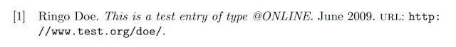
With the BibTeX entry


@ONLINE{Doe:2009:Online,
author = {Doe, Ringo},
title = {This is a test entry of type {@ONLINE}},
month = jun,
year = {2009},
url = {http://www.test.org/doe/}
}

and the LaTeX file


\documentclass{article}

\usepackage{biblatex}
\bibliography{test. bib}

\title{BibTeX Website citatations with the \textsf{biblatex}~package}
\date{}

\begin{document}

\maketitle
\nocite{Doe:2009:Online}
\printbibliography

\end{document}

one gets a nicely typeset list of references.

Note that there are plenty of more options and entry types in the biblatex package, such as (the currently unused)
@AUDIO and 
@VIDEO.

Because of its supposedly large impact on the (La)TeX community, the author of biblatex still declares the package as ‘beta’ which is why it is not included in TeXlive, for example. Should you for this or some other reason be unable to install biblatex, there are (inferior) alternatives to use for URL citations in a reference list.

Alternatives
Using the natbib package The natbib package extends the functionality of regular bibtex to a certain degree, and allows for website citations as well. There is no specific entry type for online resources, but 
@MISC
@OTHER, and 
@BOOKLET work quite well.


@BOOKLET{Doe:2009:Booklet,
title = {This is a test entry of type {@BOOKLET}},
author = {Doe, John},
month = jun,
year = {2009},
url = {http://www.test.org/doe/}
}

@MISC{Doe:2009:Misc,
author = {Doe, Paul},
title = {This is a test test entry of type {@MISC}},
month = jun,
year = {2009},
url = {http://www.test.org/doe/}
}

@OTHER{Doe:2009:Other,
author = {Doe, Brian},
title = {This is a test entry of type {@OTHER}},
month = jun,
year = {2009},
url = {http://www.test.org/doe/}
}

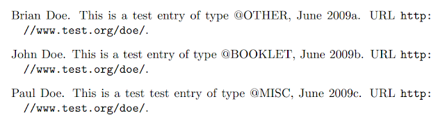
Note that standard bibstyles (such as 
plain) will not typeset the 
url key contents of the individual entries; it is required to use one of natbib’s own entries, e.g. 
plainnat.


\documentclass{article}

\usepackage{natbib}
\bibliographystyle{plainnat}

\usepackage{url}

\title{BibTeX Website citations with the \textsf{natbib} package}
\date{}

\begin{document}

\maketitle
\nocite{Doe:2009:Other,
Doe:2009:Misc,
Doe:2009:Booklet}
\bibliography{test}

\end{document}

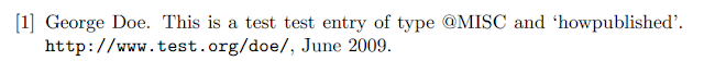
Using the url package The most elemental way to include web references is via the 
howpublished key of the 
@MISC entry. Use

@MISC{Doe:2009:Misc,
author = {Doe, George},
title = {This is a test test entry of type {@MISC} and `howpublished'},
month = jun,
year = {2009},
howpublished={\url{http://www.test.org/doe/}}
}

and

\documentclass{article}
\bibliographystyle{plain}

\usepackage{url}

\begin{document}

\nocite{Doe:2009:Misc}
\bibliography{mybib}

\end{document}


R language – path setting and working directory modification

Path setting in R language
Software path setting is important for memory management, working data storage, and getting to the bottom of things. Therefore, a reasonable setting of the relevant path in R can facilitate the management of relevant documents, improve the efficiency of learning R language, and establish their own habit system.
The path setting in R mainly includes the following aspects:
Path to the working directory Path to the installation package


Working directory
1. Use the geTWd () function to display the current working directory;

getwd()

2. Change the current directory using the seTWd () function;

setwd("D:/R")

Note: the
(1) function setwd() does not automatically create a directory that does not exist. If necessary, you can use the function dir. Create () to create a new directory, then use setwd() to point the working directory to the new directory.
(2) Dir. Create () in R is non-cascading, meaning that only one “/” path can be created at a time. If you need two “/” paths, you need to create them twice with dir. Create () before the file is created successfully. Then follow the example and use seTWd () to set it.
(3) The seTWd () function is to set a temporary work path. 3. Use the RStudio window to permanently change the working directory
A.
B.

 
Package installation
Once and for all: (Run RStudio as administrator) write the following command in R:

.libPaths("C:/Program Files/R/R-3.5.2/library")

or
Run RStudio as an administrator