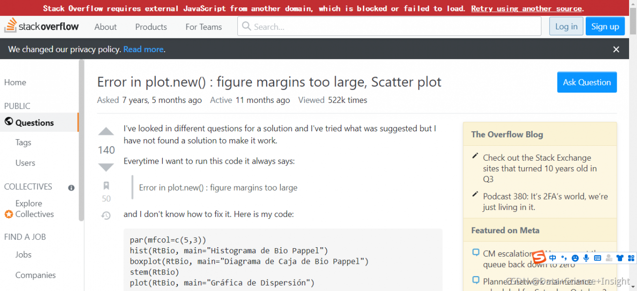
Error in plot.new() : figure margins too large
Full error:
#Question
Fit the regression model and calculate the dfbetas value of each sample and the optimal dfbetas threshold. Finally, visualize the impact of each sample on each predictive variable;
#fit a regression model
model <- lm(mpg~disp+hp, data=mtcars)

#view model summary
summary(model)

#calculate DFBETAS for each observation in the model
dfbetas <- as.data.frame(dfbetas(model))

#display DFBETAS for each observation
dfbetas

#find number of observations
n <- nrow(mtcars)

#calculate DFBETAS threshold value
thresh <- 2/sqrt(n)

thresh

#specify 2 rows and 1 column in plotting region

#dev.off()
#par(mar = c(1, 1, 1, 1))

par(mfrow=c(2,1))

#plot DFBETAS for disp with threshold lines
plot(dfbetas$disp, type='h')
abline(h = thresh, lty = 2)
abline(h = -thresh, lty = 2)

#plot DFBETAS for hp with threshold lines
plot(dfbetas$hp, type='h')
abline(h = thresh, lty = 2)
abline(h = -thresh, lty = 2)
#Solution
par(mar = c(1, 1, 1, 1))
#fit a regression model
model <- lm(mpg~disp+hp, data=mtcars)

#view model summary
summary(model)

#calculate DFBETAS for each observation in the model
dfbetas <- as.data.frame(dfbetas(model))

#display DFBETAS for each observation
dfbetas

#find number of observations
n <- nrow(mtcars)

#calculate DFBETAS threshold value
thresh <- 2/sqrt(n)

thresh

#specify 2 rows and 1 column in plotting region

#dev.off()
par(mar = c(1, 1, 1, 1))

par(mfrow=c(2,1))

#plot DFBETAS for disp with threshold lines
plot(dfbetas$disp, type='h')
abline(h = thresh, lty = 2)
abline(h = -thresh, lty = 2)

#plot DFBETAS for hp with threshold lines
plot(dfbetas$hp, type='h')
abline(h = thresh, lty = 2)
abline(h = -thresh, lty = 2)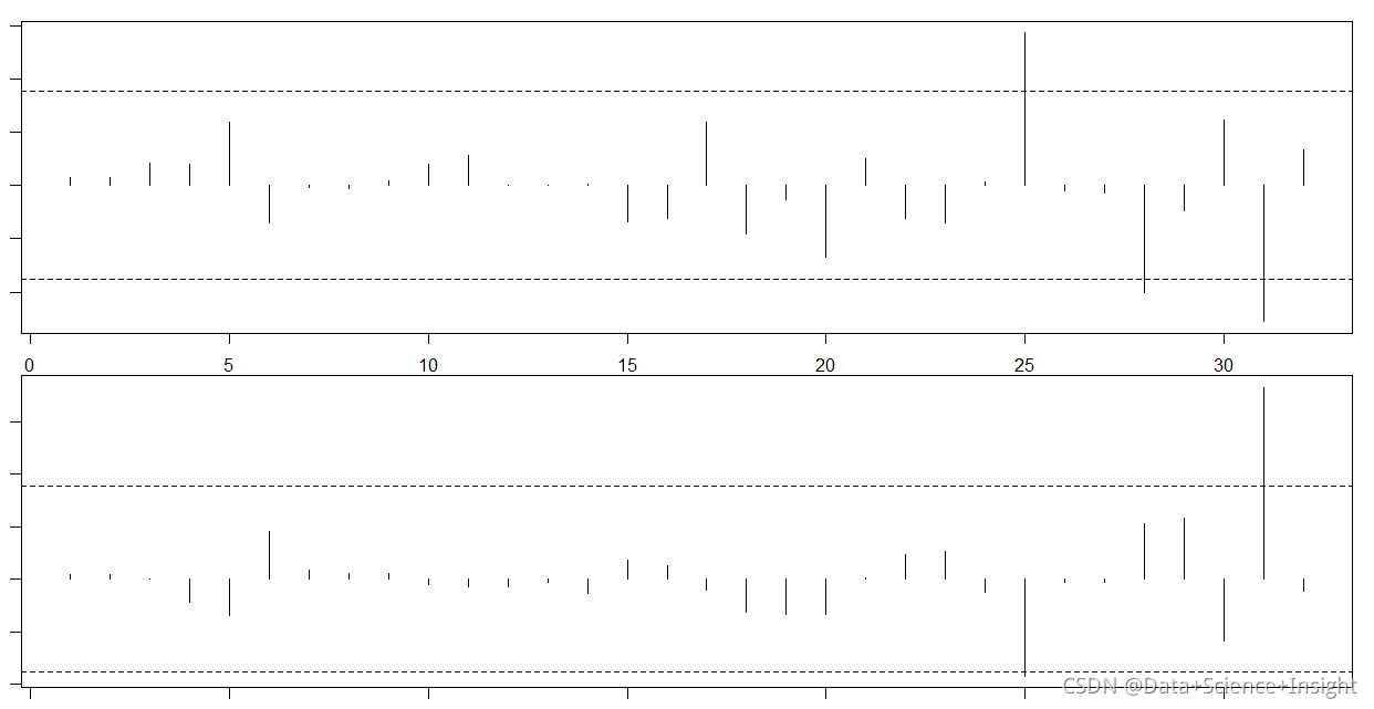
Full Error Message:
> par(mfrow=c(2,1))
>
> #plot DFBETAS for disp with threshold lines
> plot(dfbetas$disp, type=’h’)
Error in plot.new() : figure margins too large
> abline(h = thresh, lty = 2)
Error in int_abline(a = a, b = b, h = h, v = v, untf = untf, …) :
plot.new has not been called yet
> abline(h = -thresh, lty = 2)
Error in int_abline(a = a, b = b, h = h, v = v, untf = untf, …) :
plot.new has not been called yet
>
> #plot DFBETAS for hp with threshold lines
> plot(dfbetas$hp, type=’h’)
Error in plot.new() : figure margins too large
> abline(h = thresh, lty = 2)
Error in int_abline(a = a, b = b, h = h, v = v, untf = untf, …) :
plot.new has not been called yet
> abline(h = -thresh, lty = 2)
Error in int_abline(a = a, b = b, h = h, v = v, untf = untf, …) :
plot.new has not been called yet