directory

perspective Pandas DataFrame

groups the data in Pandas DataFrame

summary

---

After using our dataset, we’ll take a quick look at visualizations that can be easily created from the dataset using the popular Python library, and then walk through an example of visualizations.

• download CSV and database file – 127.8 KB
• download the source code 122.4 KB
  

  Python and “Pandas” is part of the data cleaning series. It aims to leverage data science tools and technologies to get developers up and running quickly.

  if you would like to see other articles in this series, they can be found here:

  Part 1 – introduction to Pandas</li b>

• – loading CSV and SQL data into Pandas
• – correcting missing data
• – merging multiple data sets in Pandas
• – cleaning up Pandas part 5 – removing Pandas

• -0 1 1 2 4 5

• 6
• 7 part 7 – use seaframe and Pandas to visualize data
• 8

9
DataFrame to make the most of the data.

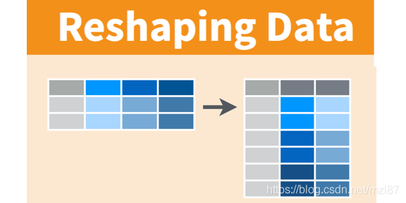
, even after the data set is cleaned up, the Pandas need to be reshaped to make the most of the data. Remodeling is manipulating the table structure to form a term used when different data sets, such as </ span> “</ span> wide </ span> ” </ span> data table is set to </ span> “</ span> long </ span> ” </ span> .

and 0 1 cross 2 3 table support, you will be familiar with this if you have used pivottability tables in or data built into many relational databases pivot and 1 cross 2 3 table support.

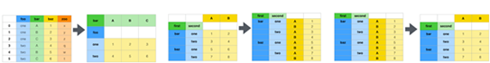
For example, the table above (Pandas document. ) has been adjusted by perspective, stacking or disassembling the table.

</ span> stack0 method takes tables with multiple indexes and groups them into groups 1 2

• 3 4 unstack6 method takes tables with multiple unique columns and ungroups them into groups 7 89in this phase, we will study a variety of methods to use to reshape the data. We’ll see how to use perspective and stack of data frames to get different images of the data.

  please note that we have used this series of module source data files to create a full , you can in the head of this article download and install .

  see through  Pandas  DataFrame

  , we can use pivot function to create a new 0 1 DataFrame2 3 from the existing frame. So far, our table has been indexed by buy ID, but let’s convert the previously created combinedData table into a more interesting table.

  First, let’s try the following

  method by starting a new code block and adding:

  productsByState = combinedData.pivot(index='product_id', columns='company', values='paid')

  the result looks something like this:

  

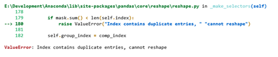
  running this command will result in a duplicate index error, only applies to DataFrame.

  but there’s another way to get us to a solution to this problem. pivot_table works similarly to PivotTable, but it will aggregate duplicate values without generating errors.

   

; pivot_table; pivot_table; pivot_table

let’s use this method with the default value:

productsByState = combinedData.pivot_table(index=['product_id', 'product'], columns='state', values='paid')

you can view the results here:

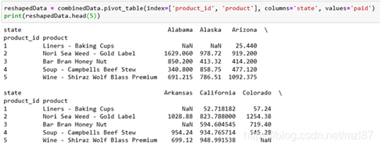
This will produce a DataFrame, which contains the list of products and the average of each state in each column. This isn’t really that useful, so let’s change the aggregation method:

reshapedData = combinedData.pivot_table(index=['product_id', 'product'], columns='state', values='paid', aggfunc=np.sum)
reshapedData = reshapedData.fillna(0)
print(reshapedData.head(10))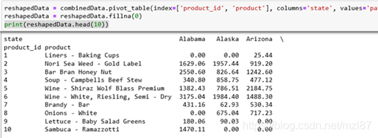

now, this will generate a product table that contains the total sales of all these products in each state. The second line of this method also removes the NaN value and replaces it with 0, since it is assumed that the product is not sold in this state.

in to group data

another remodeling activity that we’ll see is grouping data elements together. Let’s go back to the original large DataFrame and create a new DataFrame.

• groupby </ span> method the large data set and grouped according to the column value </ span> </ li> </ ul>
  Start a new code block and add:

volumesData = combinedData.groupby(by='customer_id') print(volumesData.head(10))

results as follows:

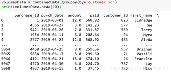
doesn’t seem to be really doing anything because our DataFrame was on purchase_id.

let’s add a summary function to summarize the data so that our grouping works as expected:

volumesData = combinedData.groupby(by='customer_id').sum()
print(volumesData.head(10))

again, this is the result:

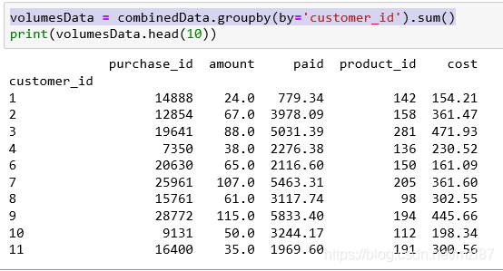
this would group the data set the way we expected but we seem to be missing some columns and doesn’t make any sense so let’s extend the groupby method and trim that 0 1 purchase_id2 3 column: 4

5

volumesData = combinedData.groupby(by=['customer_id','first_name','last_name','product_id','product']).sum()
volumesData.drop(columns='purchase_id', inplace=True)
print(volumesData.head(10))

this is our new result:

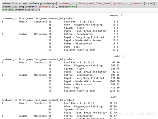
the end result looks good and gives us a good idea of what the customer is buying, the amount of money and how much they are paying.

Finally, we will make another change to the groupby data set. Add the following to create a total for each state DataFrame :

totalsData = combinedData.groupby(by='state').sum().reset_index()
totalsData.drop(columns=['purchase_id','customer_id','product_id'], inplace=True)

The key change here is that we added a sum after the reset_index. This is to ensure that the generated DataFrame has available indexes for our visualization work.

summary

we have taken a complete, clean data set and adapted it in several different ways to give us more insight into the data.

Next, we’ll look at visualizations and see how they can be an important tool for presenting our data and ensuring that the results are clean.