1. Solve function

This is the simplest way to solve differential equations – symbolic solution. Generally speaking, there are two methods to solve ordinary differential equations in MATLAB, one is symbolic solution, the other is numerical solution. In the undergraduate stage of differential mathematics problems, basically can be solved by symbolic solution.

The key command of symbolic solution to ordinary differential problem with MATLAB is dslove command. In this command, D can be used to represent the differential symbol, where D2 represents the second order differential, D3 represents the third order differential, and so on. It is worth noting that the differential is derived from the independent variable t by default, and it can be easily changed to other variables in the command.

① Seeking analytic solution

y’‘= a*y+ bx;

s = dsolve(‘D2y=a*y+b*x’,’x’);

D2y is used to represent the second derivative of Y. by default, t is the independent variable, so it is better to indicate that the independent variable is X

 

② Initial value problem

y’ = y – 2*t / y , y(0) = 1;

s = dsolve(‘Dy == y – 2*t / y’,’y(0) ==1′);

 

③ Boundary value problem

x*y’’ – 3*y’ = x^2 , y(1) = 0 , y(5) = 0;

s = dsolve(‘x*D2y – 3*Dy ==x^2′,’y(1)=0′,’y(5) == 0′,’x’);

The last argument to the function indicates that the argument is X

 

④ Higher order equation

The solution is y ‘= cos (2x) – y, y (0) = 1, y’ (0) = 0;

s=dsolve(‘D2y == cos(2*x) – y’,’y(0) =1′,’Dy(0) = 0′,’x’);

simplify(s);

 

⑤ System of equations problem

f’ = f + g , g’ = -f + g,f(0) = 1, g(0) =2;

[f,g]= dsolve(‘Df == f + g’,’Dg = -f + g’,’f(0)==1′,’g(0) == 2′,’x’);

 

 

In addition, for linear differential equations with constant coefficients, especially for higher-order linear differential equations with constant coefficients, the fundamental solutions of the corresponding homogeneous differential equations can be obtained by the eigenvalue method, and then the special solutions can be obtained by the constant variation method.

For example:

The general solution of X ” + 0.2x ‘+ 3.92x = 0

Solution: the characteristic equation is: x ^ 2 + 0.2x + 3.92 = 0

roots( [ 1 0.2 3.92 ] )  

Then work it out and keep doing it.

 

 

 

2.ode45

The common format [T, y] = ode45 (odefun, tspan, Y0)
is as follows:

odefun	is used to represent the function handle or inline function I of F (T, y), where t is scalar and Y is scalar or vector
tspan	if it is a two-dimensional vector [T0, TF], it represents the initial value t0 and final value TF of the independent variable; if it is a high-dimensional vector [T0, T1, The output node column vector (T0, T1,…, TN) ^ t
Y0	initial value vector Y0
T	represents the node column vector (T0, T1,…, TN) ^ t
y	numerical solution matrix, and each column corresponds to a component of Y

 

Ode is the most commonly used instruction to solve differential equations. It adopts variable step Runge Kutta felhberg method of fourth and fifth order, which is suitable for high accuracy problems. Ode23 is similar to ode45, but its accuracy is lower.

 

For example:

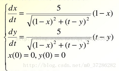
1. Create a function file eq2. M to describe the differential equations of the solution in the function file

%eq2.m File
% Describe the system of differential equations

function dy=eq2(t,y) 
 % illustrate that the differential variables are two-dimensional, such that y(1)=x,y(2)=y
dy=zeros(2,1); 
% System of differential equations
dy(1)=5*(1-y(1))/sqrt((1-y(1))^2+(t-y(2))^2);
dy(2)=5*(1-y(2))/sqrt((1-y(1))^2+(t-y(2))^2);
end

 

2. Call ode45 function to solve differential equations

[t,y]=ode45(@eq2,[0,2],[0,0]);

 

Ode45 Function Description: the first parameter is the name of the equation, the second parameter is the range of T when solving, and the third group of parameters is the initial value of each element in y.

[t,y]=ode45(@eq2,[t1,t2],[y1(0),y2(0)]);

 

Part of it comes from http://blog.csdn.net/qq_ 28093585/article/details/70276454。