Tag Archives: Experience of Using Matlab

Matlab: Three forms of random number generated (Rand, Randi and Randn)

There are three kinds of library functions about random number generation in MATLAB. Let’s take a look at their forms:
1, Rand (…) 
it is to generate pseudo-random numbers with uniform distribution between 0 and 1 (open-loop, excluding 0 and 1), that is, infinite tests, in which the probability of each number is the same.
its function format is as follows:

 R = rand(N)              % Generate an N×N matrix of random numbers, where each element lies between 0 and 1
 R = rand([M,N,P,...])    % Generate M×N×P×... of matrix random numbers
 R = rand(M,N,P,...)      % As above, the brackets are not required
 R = rand(... , CLASSNAME) % Generate a random number of type CLASSNAME, e.g. 'double' or 'single' 

for example, generate a double type of 5 × 3 evenly distributed random number between 0 and 1:

R = rand(5,3,'double');

similarly, we want to generate 100 data between [a, b], which can be expressed as:

R = a + (b-a).*rand(100,1);

2.randi(…)
Randi (n) is a pseudo-random number evenly distributed among the generated (0, n), and the numbers are all integers, so each number is between 1 and n. It can be expressed in the following ways:

R = randi(iMax)            % Generate a uniformly distributed random number between 1:iMax
R = randi(iMax,m,n) % Generate a uniformly distributed random number between 1:iMax for m×n
R = randi([iMin,iMax],m,n) % Generate a uniformly distributed random number between iMin:iMax for m×n

for example:

R1 = randi(10,5,1); % Generate a 5×1 random number between 1:10
R2 = randi([10,20],2,3); % Generate a 2×3 random number between 10:20

3.randn(… )
sometimes we want to generate random numbers with normal distribution instead of random distribution, so we need to use randn function. The overall probability of the random number generated by it is normal distribution, the mean value is 0, and the variance is 1. That is to say, the probability of 0 in the generated number is the largest, and the more infinite or negative infinite the probability is smaller, but the random number may be all real numbers, but the probability of occurrence is different. Its format is as follows:

R = randn(N)   % Generate N x N normally distributed random numbers
R = randn(M,N) % Generate M×N normally distributed random numbers

for example:

R = randi(3); % Generate 3×3 normally distributed random numbers

4. Stable restart distribution RNG
here, let’s see how to make the random number generated by each program run the same, mainly with the help of the Lang function, and the format is as follows: 1

rng('default');
R = rand(1,5); % Generate a constant 1×5 random number per program run

in addition, there are expressions that generate the same distribution:

s = rng;
R1 = rand(1,5);
rng(s);
R2 = rand(1,5); % R1 and R2 random numbers are the same
How to Solve differential equations with MATLAB

1. Solve function

This is the simplest way to solve differential equations – symbolic solution. Generally speaking, there are two methods to solve ordinary differential equations in MATLAB, one is symbolic solution, the other is numerical solution. In the undergraduate stage of differential mathematics problems, basically can be solved by symbolic solution.

The key command of symbolic solution to ordinary differential problem with MATLAB is dslove command. In this command, D can be used to represent the differential symbol, where D2 represents the second order differential, D3 represents the third order differential, and so on. It is worth noting that the differential is derived from the independent variable t by default, and it can be easily changed to other variables in the command.

① Seeking analytic solution

y’‘= a*y+ bx;

s = dsolve(‘D2y=a*y+b*x’,’x’);

D2y is used to represent the second derivative of Y. by default, t is the independent variable, so it is better to indicate that the independent variable is X


② Initial value problem

y’ = y – 2*t / y , y(0) = 1;

s = dsolve(‘Dy == y – 2*t / y’,’y(0) ==1′);


③ Boundary value problem

x*y’’ – 3*y’ = x^2 , y(1) = 0 , y(5) = 0;

s = dsolve(‘x*D2y – 3*Dy ==x^2′,’y(1)=0′,’y(5) == 0′,’x’);

The last argument to the function indicates that the argument is X


④ Higher order equation

The solution is y ‘= cos (2x) – y, y (0) = 1, y’ (0) = 0;

s=dsolve(‘D2y == cos(2*x) – y’,’y(0) =1′,’Dy(0) = 0′,’x’);

simplify(s);


⑤ System of equations problem

f’ = f + g , g’ = -f + g,f(0) = 1, g(0) =2;

[f,g]= dsolve(‘Df == f + g’,’Dg = -f + g’,’f(0)==1′,’g(0) == 2′,’x’);


In addition, for linear differential equations with constant coefficients, especially for higher-order linear differential equations with constant coefficients, the fundamental solutions of the corresponding homogeneous differential equations can be obtained by the eigenvalue method, and then the special solutions can be obtained by the constant variation method.

For example:

The general solution of X ” + 0.2x ‘+ 3.92x = 0

Solution: the characteristic equation is: x ^ 2 + 0.2x + 3.92 = 0

roots( [ 1 0.2 3.92 ] )  

Then work it out and keep doing it.


2.ode45

The common format [T, y] = ode45 (odefun, tspan, Y0)
is as follows:

odefun is used to represent the function handle or inline function I of F (T, y), where t is scalar and Y is scalar or vector
tspan if it is a two-dimensional vector [T0, TF], it represents the initial value t0 and final value TF of the independent variable; if it is a high-dimensional vector [T0, T1, The output node column vector (T0, T1,…, TN) ^ t
Y0 initial value vector Y0
T represents the node column vector (T0, T1,…, TN) ^ t
y numerical solution matrix, and each column corresponds to a component of Y


Ode is the most commonly used instruction to solve differential equations. It adopts variable step Runge Kutta felhberg method of fourth and fifth order, which is suitable for high accuracy problems. Ode23 is similar to ode45, but its accuracy is lower.


For example:

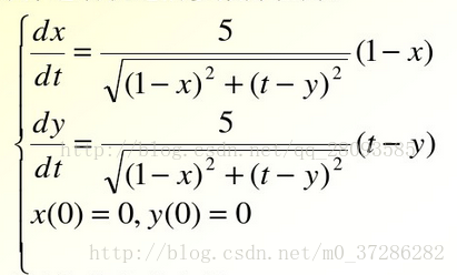
1. Create a function file eq2. M to describe the differential equations of the solution in the function file

%eq2.m File
% Describe the system of differential equations

function dy=eq2(t,y) 
 % illustrate that the differential variables are two-dimensional, such that y(1)=x,y(2)=y
dy=zeros(2,1); 
% System of differential equations
dy(1)=5*(1-y(1))/sqrt((1-y(1))^2+(t-y(2))^2);
dy(2)=5*(1-y(2))/sqrt((1-y(1))^2+(t-y(2))^2);
end


2. Call ode45 function to solve differential equations

[t,y]=ode45(@eq2,[0,2],[0,0]);


Ode45 Function Description: the first parameter is the name of the equation, the second parameter is the range of T when solving, and the third group of parameters is the initial value of each element in y.

[t,y]=ode45(@eq2,[t1,t2],[y1(0),y2(0)]);


Part of it comes from http://blog.csdn.net/qq_ 28093585/article/details/70276454。