Author Archives: Robins

How to Disable Autoconfiguration IPv4 Address

To fix it, enter these from Command Prompt:

C:\Users\lyngtinh> netsh interface ipv4 show inter

result as:

Idx Met MTU State Name

— ———- ———- ———— —————————

1 50 4294967295 connected Loopback Pseudo-Interface 1

11
10 1500 connected Local Area Connection

11: <=Keep it in mind

Next run this command:

C:\Users\lyngtinh>netsh interface ipv4 set interface
11 dadtransmits=0 store=persistent

Next, enter

Run > services.msc
> disable DHCP Client service

Final, restart your server.

Good luck!

The Use of Minimize Function (cipy.optimize)

The use of the minimize function
1. How to view the function 2. Minimize function in search of parameters 3. Minimize the solution of the constraint function. 4

1. How do I view functions
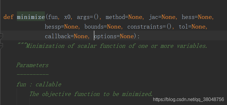
To view a function in Python, press Ctrl and then mouse click or Ctrl+B to jump to the definition of the function, which also contains the example used by the function.

2. The search for parameters is a minimize function
I come into contact with Wu En fminunc function is looking at video of machine learning, for the use of the function in matlab: the need to define a costFunction (theta), calculate the loss function and gradient in the function, will return the value of the two, then the function address, initial theta, and options to fminunct function, then the function will return theta and the optimized value loss, and exitFlag (the value 1 represents the convergence, 0) convergence. This function will automatically select conjugate gradient, BFGS and one of the L-BFGS algorithms to automatically select the learning rate, so as to optimize the gradient descent function.
Minimize (). The use of this function is a little different from MATLAB’s fminunc function. Here’s a summary of the problems you run into in using it.
1. First check the function:
official statement is too long, I put it at the end of this blog post:

//Here's the declaration. I think it's a good idea to check the function's description.
def minimize(fun, x0, args=(), method=None, jac=None, hess=None,
             hessp=None, bounds=None, constraints=(), tol=None,
             callback=None, options=None):

fun : this parameter is the costFunction that you want to minimize the loss of. Pass the name of costFunction to fun
.
The objective function to be minimized.
fun(x, *args) -> float
where x is an 1-D array with shape (n,) and args
is a tuple of the fixed parameters needed to completely
specify the function.
This means that when the loss function is defined, ** must be the first argument and its shape must be (n,)**, a one-dimensional array. Other parameters used in the calculation of the loss function are passed into the args parameters (other parameters specifically refer to X, Y, lambda, etc.) in the form of tuples, and finally return the loss value, which can be in the form of an array or a real number.
The parameter x0 is initialized to theta, whose shape must be shape(n,), which is a one-dimensional array.
method : this parameter represents the way to be adopted, default is one of BFGS, l-bfgs-b , SLSQP, optional TNC
jac : this parameter is a function to calculate the gradient. Similar to the fun parameter, the first parameter must be theta and its shape must be (n,), which is a one-dimensional array. The gradient returned at the end must also be a one-dimensional array.
options : used to control the maximum number of iterations and set in the form of a dictionary, for example: options={‘ maxiter ‘:400}
The parameters used are mainly these, and the application examples are as follows (where Ng’s machine learning EX2 is used) :

def costFunction(theta,X,Y,lmd):
    theta = theta.reshape((len(theta), 1))
    Y=Y.reshape(len(Y),1)
    m=X.shape[0]
    J=0
    first=-(Y.T)@np.log(sigmoid(X@theta))
    second=(1-Y.T)@np.log(1-sigmoid(X@theta))
    theta2=theta[1:,:]
    assert (theta2.shape==(theta.size-1,1))
    J=(first-second)/m+lmd/(2*m)*(theta2.T@theta2)
    return J
def gradient(theta,X,Y,lmd):
    theta = theta.reshape((len(theta), 1))
    Y = Y.reshape(len(Y), 1)
    reg = (lmd/len(X)) * theta
    reg[0] = 0
    grad=(X.T @ (sigmoid(X @ theta) - Y))/len(X)
    return (grad+reg).ravel()

result=op.minimize(fun=costFunction,x0=theta.reshape(28,),args=(X,Y,1),method='TNC',jac=gradient,options={'maxiter':400})
print(result)
final_theta = result.x
Output:
fun: array([[0.52900273]])
     jac: array([-2.15010332e-06,  6.79564299e-07, -3.48680372e-07,  8.76012223e-07,
       -4.07509002e-08, -9.33423708e-07, -5.14520466e-07,  1.71377727e-08,
        1.55330746e-08, -9.72472529e-07,  6.96683054e-08,  3.55303286e-08,
       -2.79411735e-07,  1.79649627e-07,  2.33480997e-07,  1.47186558e-07,
       -2.11705227e-07,  6.16713286e-07, -9.29181534e-08, -5.27541662e-08,
       -1.48146987e-06,  2.31241473e-07,  1.80347588e-07, -1.31898660e-07,
       -7.16759904e-08, -4.12328300e-07,  1.65360544e-08, -7.34643861e-07])
 message: 'Converged (|f_n-f_(n-1)| ~= 0)'
    nfev: 32
     nit: 7
  status: 1
 success: True
       x: array([ 1.27271027,  0.62529965,  1.18111686, -2.019874  , -0.91743189,
       -1.4316693 ,  0.12393227, -0.36553118, -0.35725403, -0.17516292,
       -1.45817009, -0.05098418, -0.61558553, -0.27469166, -1.19271298,
       -0.2421784 , -0.20603297, -0.04466178, -0.27778952, -0.29539513,
       -0.45645982, -1.04319155,  0.02779373, -0.29244871,  0.0155576 ,
       -0.32742406, -0.1438915 , -0.92467487])

1. The X0 parameter is the initialized theta, which must be a one-dimensional array, and the gradient return value must be a one-dimensional array, i.e., the gradient is stored as a one-dimensional array.
2. An array using the attention to the shape, to learn how to reasonable use reshape make sure it is operating. 3. For one-dimensional array a=[0,1,2,3], a[0]. Shape =(), a[0]. Size =1.
3. Minimize the solution of constraint functions
Fun: To find the minimum target function
X0: The initial guess for the variable. If there are multiple variables, you need to give each one an initial guess. Minimize the occurrence of local optimality, so it is necessary to find a means of dealing with it.
Args: constant values, as will be explained in the following examples. There are no Numbers in FUN, but they are expressed in the form of variables. For constant terms, we need to give a value here
Method: There are many ways to find an extreme value. The default is generally used. Each method I understand is to calculate the error, the way of back propagation is different, this area has a lot of theoretical research space
Constraints: Constraints that constrain the part of FUN that is the parameter

1.Calculate the minimum value of 1/x+x

# coding=utf-8
from scipy.optimize import minimize
import numpy as np
 
#demo 1
#Calculate the minimum value of 1/x+x
 def fun(args):
     a=args
     v=lambda x:a/x[0] +x[0]
     return v
 
 if __name__ == "__main__":
     args = (1)  #a
     x0 = np.asarray((2))  # Initial guesses
     res = minimize(fun(args), x0, method='SLSQP')
     print(res.fun)
     print(res.success)
     print(res.x)

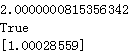
Results: the function of the minimum value for more than 2 points
the block reference link: https://blog.csdn.net/ljyljyok/article/details/100552618
4. It is a minimize function
Scipy api:https://docs.scipy.org/doc/scipy-0.18.1/reference/index.html

"""
Unified interfaces to minimization algorithms.

Functions
---------
- minimize : minimization of a function of several variables.
- minimize_scalar : minimization of a function of one variable.
"""
from __future__ import division, print_function, absolute_import


__all__ = ['minimize', 'minimize_scalar']


from warnings import warn

import numpy as np

from scipy._lib.six import callable

from scipy.sparse.linalg import LinearOperator

# unconstrained minimization
from .optimize import (_minimize_neldermead, _minimize_powell, _minimize_cg,
                       _minimize_bfgs, _minimize_newtoncg,
                       _minimize_scalar_brent, _minimize_scalar_bounded,
                       _minimize_scalar_golden, MemoizeJac)
from ._trustregion_dogleg import _minimize_dogleg
from ._trustregion_ncg import _minimize_trust_ncg
from ._trustregion_krylov import _minimize_trust_krylov
from ._trustregion_exact import _minimize_trustregion_exact
from ._trustregion_constr import _minimize_trustregion_constr
from ._constraints import Bounds, new_bounds_to_old, old_bound_to_new


# constrained minimization
from .lbfgsb import _minimize_lbfgsb
from .tnc import _minimize_tnc
from .cobyla import _minimize_cobyla
from .slsqp import _minimize_slsqp


def minimize(fun, x0, args=(), method=None, jac=None, hess=None,
             hessp=None, bounds=None, constraints=(), tol=None,
             callback=None, options=None):
    """Minimization of scalar function of one or more variables.

    Parameters
    ----------
    fun : callable
        The objective function to be minimized.

            ``fun(x, *args) -> float``

        where x is an 1-D array with shape (n,) and `args`
        is a tuple of the fixed parameters needed to completely
        specify the function.
    x0 : ndarray, shape (n,)
        Initial guess. Array of real elements of size (n,),
        where 'n' is the number of independent variables.
    args : tuple, optional
        Extra arguments passed to the objective function and its
        derivatives (`fun`, `jac` and `hess` functions).
    method : str or callable, optional
        Type of solver.  Should be one of

            - 'Nelder-Mead' :ref:`(see here) <optimize.minimize-neldermead>`
            - 'Powell'      :ref:`(see here) <optimize.minimize-powell>`
            - 'CG'          :ref:`(see here) <optimize.minimize-cg>`
            - 'BFGS'        :ref:`(see here) <optimize.minimize-bfgs>`
            - 'Newton-CG'   :ref:`(see here) <optimize.minimize-newtoncg>`
            - 'L-BFGS-B'    :ref:`(see here) <optimize.minimize-lbfgsb>`
            - 'TNC'         :ref:`(see here) <optimize.minimize-tnc>`
            - 'COBYLA'      :ref:`(see here) <optimize.minimize-cobyla>`
            - 'SLSQP'       :ref:`(see here) <optimize.minimize-slsqp>`
            - 'trust-constr':ref:`(see here) <optimize.minimize-trustconstr>`
            - 'dogleg'      :ref:`(see here) <optimize.minimize-dogleg>`
            - 'trust-ncg'   :ref:`(see here) <optimize.minimize-trustncg>`
            - 'trust-exact' :ref:`(see here) <optimize.minimize-trustexact>`
            - 'trust-krylov' :ref:`(see here) <optimize.minimize-trustkrylov>`
            - custom - a callable object (added in version 0.14.0),
              see below for description.

        If not given, chosen to be one of ``BFGS``, ``L-BFGS-B``, ``SLSQP``,
        depending if the problem has constraints or bounds.
    jac : {callable,  '2-point', '3-point', 'cs', bool}, optional
        Method for computing the gradient vector. Only for CG, BFGS,
        Newton-CG, L-BFGS-B, TNC, SLSQP, dogleg, trust-ncg, trust-krylov,
        trust-exact and trust-constr. If it is a callable, it should be a
        function that returns the gradient vector:

            ``jac(x, *args) -> array_like, shape (n,)``

        where x is an array with shape (n,) and `args` is a tuple with
        the fixed parameters. Alternatively, the keywords
        {'2-point', '3-point', 'cs'} select a finite
        difference scheme for numerical estimation of the gradient. Options
        '3-point' and 'cs' are available only to 'trust-constr'.
        If `jac` is a Boolean and is True, `fun` is assumed to return the
        gradient along with the objective function. If False, the gradient
        will be estimated using '2-point' finite difference estimation.
    hess : {callable, '2-point', '3-point', 'cs', HessianUpdateStrategy},  optional
        Method for computing the Hessian matrix. Only for Newton-CG, dogleg,
        trust-ncg,  trust-krylov, trust-exact and trust-constr. If it is
        callable, it should return the  Hessian matrix:

            ``hess(x, *args) -> {LinearOperator, spmatrix, array}, (n, n)``

        where x is a (n,) ndarray and `args` is a tuple with the fixed
        parameters. LinearOperator and sparse matrix returns are
        allowed only for 'trust-constr' method. Alternatively, the keywords
        {'2-point', '3-point', 'cs'} select a finite difference scheme
        for numerical estimation. Or, objects implementing
        `HessianUpdateStrategy` interface can be used to approximate
        the Hessian. Available quasi-Newton methods implementing
        this interface are:

            - `BFGS`;
            - `SR1`.

        Whenever the gradient is estimated via finite-differences,
        the Hessian cannot be estimated with options
        {'2-point', '3-point', 'cs'} and needs to be
        estimated using one of the quasi-Newton strategies.
        Finite-difference options {'2-point', '3-point', 'cs'} and
        `HessianUpdateStrategy` are available only for 'trust-constr' method.
    hessp : callable, optional
        Hessian of objective function times an arbitrary vector p. Only for
        Newton-CG, trust-ncg, trust-krylov, trust-constr.
        Only one of `hessp` or `hess` needs to be given.  If `hess` is
        provided, then `hessp` will be ignored.  `hessp` must compute the
        Hessian times an arbitrary vector:

            ``hessp(x, p, *args) ->  ndarray shape (n,)``

        where x is a (n,) ndarray, p is an arbitrary vector with
        dimension (n,) and `args` is a tuple with the fixed
        parameters.
    bounds : sequence or `Bounds`, optional
        Bounds on variables for L-BFGS-B, TNC, SLSQP and
        trust-constr methods. There are two ways to specify the bounds:

            1. Instance of `Bounds` class.
            2. Sequence of ``(min, max)`` pairs for each element in `x`. None
               is used to specify no bound.

    constraints : {Constraint, dict} or List of {Constraint, dict}, optional
        Constraints definition (only for COBYLA, SLSQP and trust-constr).
        Constraints for 'trust-constr' are defined as a single object or a
        list of objects specifying constraints to the optimization problem.
        Available constraints are:

            - `LinearConstraint`
            - `NonlinearConstraint`

        Constraints for COBYLA, SLSQP are defined as a list of dictionaries.
        Each dictionary with fields:

            type : str
                Constraint type: 'eq' for equality, 'ineq' for inequality.
            fun : callable
                The function defining the constraint.
            jac : callable, optional
                The Jacobian of `fun` (only for SLSQP).
            args : sequence, optional
                Extra arguments to be passed to the function and Jacobian.

        Equality constraint means that the constraint function result is to
        be zero whereas inequality means that it is to be non-negative.
        Note that COBYLA only supports inequality constraints.
    tol : float, optional
        Tolerance for termination. For detailed control, use solver-specific
        options.
    options : dict, optional
        A dictionary of solver options. All methods accept the following
        generic options:

            maxiter : int
                Maximum number of iterations to perform.
            disp : bool
                Set to True to print convergence messages.

        For method-specific options, see :func:`show_options()`.
    callback : callable, optional
        Called after each iteration. For 'trust-constr' it is a callable with
        the signature:

            ``callback(xk, OptimizeResult state) -> bool``

        where ``xk`` is the current parameter vector. and ``state``
        is an `OptimizeResult` object, with the same fields
        as the ones from the return.  If callback returns True
        the algorithm execution is terminated.
        For all the other methods, the signature is:

            ``callback(xk)``

        where ``xk`` is the current parameter vector.

    Returns
    -------
    res : OptimizeResult
        The optimization result represented as a ``OptimizeResult`` object.
        Important attributes are: ``x`` the solution array, ``success`` a
        Boolean flag indicating if the optimizer exited successfully and
        ``message`` which describes the cause of the termination. See
        `OptimizeResult` for a description of other attributes.


    See also
    --------
    minimize_scalar : Interface to minimization algorithms for scalar
        univariate functions
    show_options : Additional options accepted by the solvers

    Notes
    -----
    This section describes the available solvers that can be selected by the
    'method' parameter. The default method is *BFGS*.

    **Unconstrained minimization**

    Method :ref:`Nelder-Mead <optimize.minimize-neldermead>` uses the
    Simplex algorithm [1]_, [2]_. This algorithm is robust in many
    applications. However, if numerical computation of derivative can be
    trusted, other algorithms using the first and/or second derivatives
    information might be preferred for their better performance in
    general.

    Method :ref:`Powell <optimize.minimize-powell>` is a modification
    of Powell's method [3]_, [4]_ which is a conjugate direction
    method. It performs sequential one-dimensional minimizations along
    each vector of the directions set (`direc` field in `options` and
    `info`), which is updated at each iteration of the main
    minimization loop. The function need not be differentiable, and no
    derivatives are taken.

    Method :ref:`CG <optimize.minimize-cg>` uses a nonlinear conjugate
    gradient algorithm by Polak and Ribiere, a variant of the
    Fletcher-Reeves method described in [5]_ pp.  120-122. Only the
    first derivatives are used.

    Method :ref:`BFGS <optimize.minimize-bfgs>` uses the quasi-Newton
    method of Broyden, Fletcher, Goldfarb, and Shanno (BFGS) [5]_
    pp. 136. It uses the first derivatives only. BFGS has proven good
    performance even for non-smooth optimizations. This method also
    returns an approximation of the Hessian inverse, stored as
    `hess_inv` in the OptimizeResult object.

    Method :ref:`Newton-CG <optimize.minimize-newtoncg>` uses a
    Newton-CG algorithm [5]_ pp. 168 (also known as the truncated
    Newton method). It uses a CG method to the compute the search
    direction. See also *TNC* method for a box-constrained
    minimization with a similar algorithm. Suitable for large-scale
    problems.

    Method :ref:`dogleg <optimize.minimize-dogleg>` uses the dog-leg
    trust-region algorithm [5]_ for unconstrained minimization. This
    algorithm requires the gradient and Hessian; furthermore the
    Hessian is required to be positive definite.

    Method :ref:`trust-ncg <optimize.minimize-trustncg>` uses the
    Newton conjugate gradient trust-region algorithm [5]_ for
    unconstrained minimization. This algorithm requires the gradient
    and either the Hessian or a function that computes the product of
    the Hessian with a given vector. Suitable for large-scale problems.

    Method :ref:`trust-krylov <optimize.minimize-trustkrylov>` uses
    the Newton GLTR trust-region algorithm [14]_, [15]_ for unconstrained
    minimization. This algorithm requires the gradient
    and either the Hessian or a function that computes the product of
    the Hessian with a given vector. Suitable for large-scale problems.
    On indefinite problems it requires usually less iterations than the
    `trust-ncg` method and is recommended for medium and large-scale problems.

    Method :ref:`trust-exact <optimize.minimize-trustexact>`
    is a trust-region method for unconstrained minimization in which
    quadratic subproblems are solved almost exactly [13]_. This
    algorithm requires the gradient and the Hessian (which is
    *not* required to be positive definite). It is, in many
    situations, the Newton method to converge in fewer iteraction
    and the most recommended for small and medium-size problems.

    **Bound-Constrained minimization**

    Method :ref:`L-BFGS-B <optimize.minimize-lbfgsb>` uses the L-BFGS-B
    algorithm [6]_, [7]_ for bound constrained minimization.

    Method :ref:`TNC <optimize.minimize-tnc>` uses a truncated Newton
    algorithm [5]_, [8]_ to minimize a function with variables subject
    to bounds. This algorithm uses gradient information; it is also
    called Newton Conjugate-Gradient. It differs from the *Newton-CG*
    method described above as it wraps a C implementation and allows
    each variable to be given upper and lower bounds.

    **Constrained Minimization**

    Method :ref:`COBYLA <optimize.minimize-cobyla>` uses the
    Constrained Optimization BY Linear Approximation (COBYLA) method
    [9]_, [10]_, [11]_. The algorithm is based on linear
    approximations to the objective function and each constraint. The
    method wraps a FORTRAN implementation of the algorithm. The
    constraints functions 'fun' may return either a single number
    or an array or list of numbers.

    Method :ref:`SLSQP <optimize.minimize-slsqp>` uses Sequential
    Least SQuares Programming to minimize a function of several
    variables with any combination of bounds, equality and inequality
    constraints. The method wraps the SLSQP Optimization subroutine
    originally implemented by Dieter Kraft [12]_. Note that the
    wrapper handles infinite values in bounds by converting them into
    large floating values.

    Method :ref:`trust-constr <optimize.minimize-trustconstr>` is a
    trust-region algorithm for constrained optimization. It swiches
    between two implementations depending on the problem definition.
    It is the most versatile constrained minimization algorithm
    implemented in SciPy and the most appropriate for large-scale problems.
    For equality constrained problems it is an implementation of Byrd-Omojokun
    Trust-Region SQP method described in [17]_ and in [5]_, p. 549. When
    inequality constraints  are imposed as well, it swiches to the trust-region
    interior point  method described in [16]_. This interior point algorithm,
    in turn, solves inequality constraints by introducing slack variables
    and solving a sequence of equality-constrained barrier problems
    for progressively smaller values of the barrier parameter.
    The previously described equality constrained SQP method is
    used to solve the subproblems with increasing levels of accuracy
    as the iterate gets closer to a solution.

    **Finite-Difference Options**

    For Method :ref:`trust-constr <optimize.minimize-trustconstr>`
    the gradient and the Hessian may be approximated using
    three finite-difference schemes: {'2-point', '3-point', 'cs'}.
    The scheme 'cs' is, potentially, the most accurate but it
    requires the function to correctly handles complex inputs and to
    be differentiable in the complex plane. The scheme '3-point' is more
    accurate than '2-point' but requires twice as much operations.

    **Custom minimizers**

    It may be useful to pass a custom minimization method, for example
    when using a frontend to this method such as `scipy.optimize.basinhopping`
    or a different library.  You can simply pass a callable as the ``method``
    parameter.

    The callable is called as ``method(fun, x0, args, **kwargs, **options)``
    where ``kwargs`` corresponds to any other parameters passed to `minimize`
    (such as `callback`, `hess`, etc.), except the `options` dict, which has
    its contents also passed as `method` parameters pair by pair.  Also, if
    `jac` has been passed as a bool type, `jac` and `fun` are mangled so that
    `fun` returns just the function values and `jac` is converted to a function
    returning the Jacobian.  The method shall return an ``OptimizeResult``
    object.

    The provided `method` callable must be able to accept (and possibly ignore)
    arbitrary parameters; the set of parameters accepted by `minimize` may
    expand in future versions and then these parameters will be passed to
    the method.  You can find an example in the scipy.optimize tutorial.

    .. versionadded:: 0.11.0

    References
    ----------
    .. [1] Nelder, J A, and R Mead. 1965. A Simplex Method for Function
        Minimization. The Computer Journal 7: 308-13.
    .. [2] Wright M H. 1996. Direct search methods: Once scorned, now
        respectable, in Numerical Analysis 1995: Proceedings of the 1995
        Dundee Biennial Conference in Numerical Analysis (Eds. D F
        Griffiths and G A Watson). Addison Wesley Longman, Harlow, UK.
        191-208.
    .. [3] Powell, M J D. 1964. An efficient method for finding the minimum of
       a function of several variables without calculating derivatives. The
       Computer Journal 7: 155-162.
    .. [4] Press W, S A Teukolsky, W T Vetterling and B P Flannery.
       Numerical Recipes (any edition), Cambridge University Press.
    .. [5] Nocedal, J, and S J Wright. 2006. Numerical Optimization.
       Springer New York.
    .. [6] Byrd, R H and P Lu and J. Nocedal. 1995. A Limited Memory
       Algorithm for Bound Constrained Optimization. SIAM Journal on
       Scientific and Statistical Computing 16 (5): 1190-1208.
    .. [7] Zhu, C and R H Byrd and J Nocedal. 1997. L-BFGS-B: Algorithm
       778: L-BFGS-B, FORTRAN routines for large scale bound constrained
       optimization. ACM Transactions on Mathematical Software 23 (4):
       550-560.
    .. [8] Nash, S G. Newton-Type Minimization Via the Lanczos Method.
       1984. SIAM Journal of Numerical Analysis 21: 770-778.
    .. [9] Powell, M J D. A direct search optimization method that models
       the objective and constraint functions by linear interpolation.
       1994. Advances in Optimization and Numerical Analysis, eds. S. Gomez
       and J-P Hennart, Kluwer Academic (Dordrecht), 51-67.
    .. [10] Powell M J D. Direct search algorithms for optimization
       calculations. 1998. Acta Numerica 7: 287-336.
    .. [11] Powell M J D. A view of algorithms for optimization without
       derivatives. 2007.Cambridge University Technical Report DAMTP
       2007/NA03
    .. [12] Kraft, D. A software package for sequential quadratic
       programming. 1988. Tech. Rep. DFVLR-FB 88-28, DLR German Aerospace
       Center -- Institute for Flight Mechanics, Koln, Germany.
    .. [13] Conn, A. R., Gould, N. I., and Toint, P. L.
       Trust region methods. 2000. Siam. pp. 169-200.
    .. [14] F. Lenders, C. Kirches, A. Potschka: "trlib: A vector-free
       implementation of the GLTR method for iterative solution of
       the trust region problem", https://arxiv.org/abs/1611.04718
    .. [15] N. Gould, S. Lucidi, M. Roma, P. Toint: "Solving the
       Trust-Region Subproblem using the Lanczos Method",
       SIAM J. Optim., 9(2), 504--525, (1999).
    .. [16] Byrd, Richard H., Mary E. Hribar, and Jorge Nocedal. 1999.
        An interior point algorithm for large-scale nonlinear  programming.
        SIAM Journal on Optimization 9.4: 877-900.
    .. [17] Lalee, Marucha, Jorge Nocedal, and Todd Plantega. 1998. On the
        implementation of an algorithm for large-scale equality constrained
        optimization. SIAM Journal on Optimization 8.3: 682-706.

    Examples
    --------
    Let us consider the problem of minimizing the Rosenbrock function. This
    function (and its respective derivatives) is implemented in `rosen`
    (resp. `rosen_der`, `rosen_hess`) in the `scipy.optimize`.

    >>> from scipy.optimize import minimize, rosen, rosen_der

    A simple application of the *Nelder-Mead* method is:

    >>> x0 = [1.3, 0.7, 0.8, 1.9, 1.2]
    >>> res = minimize(rosen, x0, method='Nelder-Mead', tol=1e-6)
    >>> res.x
    array([ 1.,  1.,  1.,  1.,  1.])

    Now using the *BFGS* algorithm, using the first derivative and a few
    options:

    >>> res = minimize(rosen, x0, method='BFGS', jac=rosen_der,
    ...                options={'gtol': 1e-6, 'disp': True})
    Optimization terminated successfully.
             Current function value: 0.000000
             Iterations: 26
             Function evaluations: 31
             Gradient evaluations: 31
    >>> res.x
    array([ 1.,  1.,  1.,  1.,  1.])
    >>> print(res.message)
    Optimization terminated successfully.
    >>> res.hess_inv
    array([[ 0.00749589,  0.01255155,  0.02396251,  0.04750988,  0.09495377],  # may vary
           [ 0.01255155,  0.02510441,  0.04794055,  0.09502834,  0.18996269],
           [ 0.02396251,  0.04794055,  0.09631614,  0.19092151,  0.38165151],
           [ 0.04750988,  0.09502834,  0.19092151,  0.38341252,  0.7664427 ],
           [ 0.09495377,  0.18996269,  0.38165151,  0.7664427,   1.53713523]])


    Next, consider a minimization problem with several constraints (namely
    Example 16.4 from [5]_). The objective function is:

    >>> fun = lambda x: (x[0] - 1)**2 + (x[1] - 2.5)**2

    There are three constraints defined as:

    >>> cons = ({'type': 'ineq', 'fun': lambda x:  x[0] - 2 * x[1] + 2},
    ...         {'type': 'ineq', 'fun': lambda x: -x[0] - 2 * x[1] + 6},
    ...         {'type': 'ineq', 'fun': lambda x: -x[0] + 2 * x[1] + 2})

    And variables must be positive, hence the following bounds:

    >>> bnds = ((0, None), (0, None))

    The optimization problem is solved using the SLSQP method as:

    >>> res = minimize(fun, (2, 0), method='SLSQP', bounds=bnds,
    ...                constraints=cons)

    It should converge to the theoretical solution (1.4 ,1.7).

    """
    x0 = np.asarray(x0)
    if x0.dtype.kind in np.typecodes["AllInteger"]:
        x0 = np.asarray(x0, dtype=float)

    if not isinstance(args, tuple):
        args = (args,)

    if method is None:
        # Select automatically
        if constraints:
            method = 'SLSQP'
        elif bounds is not None:
            method = 'L-BFGS-B'
        else:
            method = 'BFGS'

    if callable(method):
        meth = "_custom"
    else:
        meth = method.lower()

    if options is None:
        options = {}
    # check if optional parameters are supported by the selected method
    # - jac
    if meth in ('nelder-mead', 'powell', 'cobyla') and bool(jac):
        warn('Method %s does not use gradient information (jac).' % method,
             RuntimeWarning)
    # - hess
    if meth not in ('newton-cg', 'dogleg', 'trust-ncg', 'trust-constr',
                    'trust-krylov', 'trust-exact', '_custom') and hess is not None:
        warn('Method %s does not use Hessian information (hess).' % method,
             RuntimeWarning)
    # - hessp
    if meth not in ('newton-cg', 'dogleg', 'trust-ncg', 'trust-constr',
                    'trust-krylov', '_custom') \
       and hessp is not None:
        warn('Method %s does not use Hessian-vector product '
             'information (hessp).' % method, RuntimeWarning)
    # - constraints or bounds
    if (meth in ('nelder-mead', 'powell', 'cg', 'bfgs', 'newton-cg', 'dogleg',
                 'trust-ncg') and (bounds is not None or np.any(constraints))):
        warn('Method %s cannot handle constraints nor bounds.' % method,
             RuntimeWarning)
    if meth in ('l-bfgs-b', 'tnc') and np.any(constraints):
        warn('Method %s cannot handle constraints.' % method,
             RuntimeWarning)
    if meth == 'cobyla' and bounds is not None:
        warn('Method %s cannot handle bounds.' % method,
             RuntimeWarning)
    # - callback
    if (meth in ('cobyla',) and callback is not None):
        warn('Method %s does not support callback.' % method, RuntimeWarning)
    # - return_all
    if (meth in ('l-bfgs-b', 'tnc', 'cobyla', 'slsqp') and
            options.get('return_all', False)):
        warn('Method %s does not support the return_all option.' % method,
             RuntimeWarning)

    # check gradient vector
    if meth == 'trust-constr':
        if type(jac) is bool:
            if jac:
                fun = MemoizeJac(fun)
                jac = fun.derivative
            else:
                jac = '2-point'
        elif not callable(jac) and jac not in ('2-point', '3-point', 'cs'):
            raise ValueError("Unsupported jac definition.")
    else:
        if jac in ('2-point', '3-point', 'cs'):
            if jac in ('3-point', 'cs'):
                warn("Only 'trust-constr' method accept %s "
                     "options for 'jac'. Using '2-point' instead." % jac)
            jac = None
        elif not callable(jac):
            if bool(jac):
                fun = MemoizeJac(fun)
                jac = fun.derivative
            else:
                jac = None

    # set default tolerances
    if tol is not None:
        options = dict(options)
        if meth == 'nelder-mead':
            options.setdefault('xatol', tol)
            options.setdefault('fatol', tol)
        if meth in ('newton-cg', 'powell', 'tnc'):
            options.setdefault('xtol', tol)
        if meth in ('powell', 'l-bfgs-b', 'tnc', 'slsqp'):
            options.setdefault('ftol', tol)
        if meth in ('bfgs', 'cg', 'l-bfgs-b', 'tnc', 'dogleg',
                    'trust-ncg', 'trust-exact', 'trust-krylov'):
            options.setdefault('gtol', tol)
        if meth in ('cobyla', '_custom'):
            options.setdefault('tol', tol)
        if meth == 'trust-constr':
            options.setdefault('xtol', tol)
            options.setdefault('gtol', tol)
            options.setdefault('barrier_tol', tol)

    if bounds is not None:
        if meth == 'trust-constr':
            if not isinstance(bounds, Bounds):
                lb, ub = old_bound_to_new(bounds)
                bounds = Bounds(lb, ub)
        elif meth in ('l-bfgs-b', 'tnc', 'slsqp'):
            if isinstance(bounds, Bounds):
                bounds = new_bounds_to_old(bounds.lb, bounds.ub, x0.shape[0])

    if meth == '_custom':
        return method(fun, x0, args=args, jac=jac, hess=hess, hessp=hessp,
                      bounds=bounds, constraints=constraints,
                      callback=callback, **options)
    elif meth == 'nelder-mead':
        return _minimize_neldermead(fun, x0, args, callback, **options)
    elif meth == 'powell':
        return _minimize_powell(fun, x0, args, callback, **options)
    elif meth == 'cg':
        return _minimize_cg(fun, x0, args, jac, callback, **options)
    elif meth == 'bfgs':
        return _minimize_bfgs(fun, x0, args, jac, callback, **options)
    elif meth == 'newton-cg':
        return _minimize_newtoncg(fun, x0, args, jac, hess, hessp, callback,
                                  **options)
    elif meth == 'l-bfgs-b':
        return _minimize_lbfgsb(fun, x0, args, jac, bounds,
                                callback=callback, **options)
    elif meth == 'tnc':
        return _minimize_tnc(fun, x0, args, jac, bounds, callback=callback,
                             **options)
    elif meth == 'cobyla':
        return _minimize_cobyla(fun, x0, args, constraints, **options)
    elif meth == 'slsqp':
        return _minimize_slsqp(fun, x0, args, jac, bounds,
                               constraints, callback=callback, **options)
    elif meth == 'trust-constr':
        return _minimize_trustregion_constr(fun, x0, args, jac, hess, hessp,
                                            bounds, constraints,
                                            callback=callback, **options)
    elif meth == 'dogleg':
        return _minimize_dogleg(fun, x0, args, jac, hess,
                                callback=callback, **options)
    elif meth == 'trust-ncg':
        return _minimize_trust_ncg(fun, x0, args, jac, hess, hessp,
                                   callback=callback, **options)
    elif meth == 'trust-krylov':
        return _minimize_trust_krylov(fun, x0, args, jac, hess, hessp,
                                      callback=callback, **options)
    elif meth == 'trust-exact':
        return _minimize_trustregion_exact(fun, x0, args, jac, hess,
                                           callback=callback, **options)
    else:
        raise ValueError('Unknown solver %s' % method)


def minimize_scalar(fun, bracket=None, bounds=None, args=(),
                    method='brent', tol=None, options=None):
    """Minimization of scalar function of one variable.

    Parameters
    ----------
    fun : callable
        Objective function.
        Scalar function, must return a scalar.
    bracket : sequence, optional
        For methods 'brent' and 'golden', `bracket` defines the bracketing
        interval and can either have three items ``(a, b, c)`` so that
        ``a < b < c`` and ``fun(b) < fun(a), fun(c)`` or two items ``a`` and
        ``c`` which are assumed to be a starting interval for a downhill
        bracket search (see `bracket`); it doesn't always mean that the
        obtained solution will satisfy ``a <= x <= c``.
    bounds : sequence, optional
        For method 'bounded', `bounds` is mandatory and must have two items
        corresponding to the optimization bounds.
    args : tuple, optional
        Extra arguments passed to the objective function.
    method : str or callable, optional
        Type of solver.  Should be one of:

            - 'Brent'     :ref:`(see here) <optimize.minimize_scalar-brent>`
            - 'Bounded'   :ref:`(see here) <optimize.minimize_scalar-bounded>`
            - 'Golden'    :ref:`(see here) <optimize.minimize_scalar-golden>`
            - custom - a callable object (added in version 0.14.0), see below

    tol : float, optional
        Tolerance for termination. For detailed control, use solver-specific
        options.
    options : dict, optional
        A dictionary of solver options.

            maxiter : int
                Maximum number of iterations to perform.
            disp : bool
                Set to True to print convergence messages.

        See :func:`show_options()` for solver-specific options.

    Returns
    -------
    res : OptimizeResult
        The optimization result represented as a ``OptimizeResult`` object.
        Important attributes are: ``x`` the solution array, ``success`` a
        Boolean flag indicating if the optimizer exited successfully and
        ``message`` which describes the cause of the termination. See
        `OptimizeResult` for a description of other attributes.

    See also
    --------
    minimize : Interface to minimization algorithms for scalar multivariate
        functions
    show_options : Additional options accepted by the solvers

    Notes
    -----
    This section describes the available solvers that can be selected by the
    'method' parameter. The default method is *Brent*.

    Method :ref:`Brent <optimize.minimize_scalar-brent>` uses Brent's
    algorithm to find a local minimum.  The algorithm uses inverse
    parabolic interpolation when possible to speed up convergence of
    the golden section method.

    Method :ref:`Golden <optimize.minimize_scalar-golden>` uses the
    golden section search technique. It uses analog of the bisection
    method to decrease the bracketed interval. It is usually
    preferable to use the *Brent* method.

    Method :ref:`Bounded <optimize.minimize_scalar-bounded>` can
    perform bounded minimization. It uses the Brent method to find a
    local minimum in the interval x1 < xopt < x2.

    **Custom minimizers**

    It may be useful to pass a custom minimization method, for example
    when using some library frontend to minimize_scalar.  You can simply
    pass a callable as the ``method`` parameter.

    The callable is called as ``method(fun, args, **kwargs, **options)``
    where ``kwargs`` corresponds to any other parameters passed to `minimize`
    (such as `bracket`, `tol`, etc.), except the `options` dict, which has
    its contents also passed as `method` parameters pair by pair.  The method
    shall return an ``OptimizeResult`` object.

    The provided `method` callable must be able to accept (and possibly ignore)
    arbitrary parameters; the set of parameters accepted by `minimize` may
    expand in future versions and then these parameters will be passed to
    the method.  You can find an example in the scipy.optimize tutorial.

    .. versionadded:: 0.11.0

    Examples
    --------
    Consider the problem of minimizing the following function.

    >>> def f(x):
    ...     return (x - 2) * x * (x + 2)**2

    Using the *Brent* method, we find the local minimum as:

    >>> from scipy.optimize import minimize_scalar
    >>> res = minimize_scalar(f)
    >>> res.x
    1.28077640403

    Using the *Bounded* method, we find a local minimum with specified
    bounds as:

    >>> res = minimize_scalar(f, bounds=(-3, -1), method='bounded')
    >>> res.x
    -2.0000002026

    """
    if not isinstance(args, tuple):
        args = (args,)

    if callable(method):
        meth = "_custom"
    else:
        meth = method.lower()
    if options is None:
        options = {}

    if tol is not None:
        options = dict(options)
        if meth == 'bounded' and 'xatol' not in options:
            warn("Method 'bounded' does not support relative tolerance in x; "
                 "defaulting to absolute tolerance.", RuntimeWarning)
            options['xatol'] = tol
        elif meth == '_custom':
            options.setdefault('tol', tol)
        else:
            options.setdefault('xtol', tol)

    if meth == '_custom':
        return method(fun, args=args, bracket=bracket, bounds=bounds, **options)
    elif meth == 'brent':
        return _minimize_scalar_brent(fun, bracket, args, **options)
    elif meth == 'bounded':
        if bounds is None:
            raise ValueError('The `bounds` parameter is mandatory for '
                             'method `bounded`.')
        # replace boolean "disp" option, if specified, by an integer value, as
        # expected by _minimize_scalar_bounded()
        disp = options.get('disp')
        if isinstance(disp, bool):
            options['disp'] = 2 * int(disp)
        return _minimize_scalar_bounded(fun, bounds, args, **options)
    elif meth == 'golden':
        return _minimize_scalar_golden(fun, bracket, args, **options)
    else:
        raise ValueError('Unknown solver %s' % method)
How to Change Local Path in TFS

How to change the local path after download file from TFS source control
File -> Source Control -> Workspaces -> Choose the workspace in question and click “Edit”.

You can also use the dropdown in Source Control Explorer, or ‘tf workspace’ at a command line within the old path.
From:http://social.msdn.microsoft.com/Forums/en-US/tfsversioncontrol/thread/d0c6982f-4f5e-4b1c-830b-3af9fb127922

Installation and configuration of redis in Linux

Pure hand, reproduced please attach this website!!
Redis goes without saying, directly to dry goods, first of all, the owner of the building is using CentOS+Redis4.0.7
Redis is stored at /usr/local, so enter /usr/local first

cd /usr/local

Download the compressed package of Redis source code in the official website

wget http://download.redis.io/releases/redis-4.0.7.tar.gz

Unzip the package

tar -zxvf redis-4.0.7.tar.gz

Install Redis. After these two commands are completed, Redis is installed in /usr/local/redis

cd redis-4.0.7/src/
make
make install PREFIX=/usr/local/redis

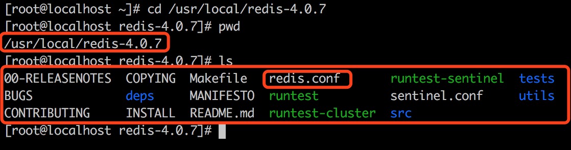
Enter the directory after installation, the building is redis-4.0.7, we will see a lot of files: redis.config is the configuration file of RedIS, which is also the file needed to start RedIS later, then enter the configuration

There are three changes to the configuration file:
1. Daemonize No should be changed to Daemonize Yes. This parameter is mainly about whether Redis should be run as a daemon process
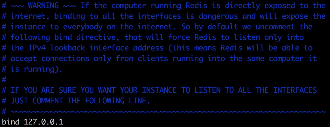
2. Change bind 127.0.0.1 to #bind 127.0.0.1 to solve the problem that the external network cannot be accessed
3, protected-mode yes change to protected-mode no to solve the problem that the external network cannot access


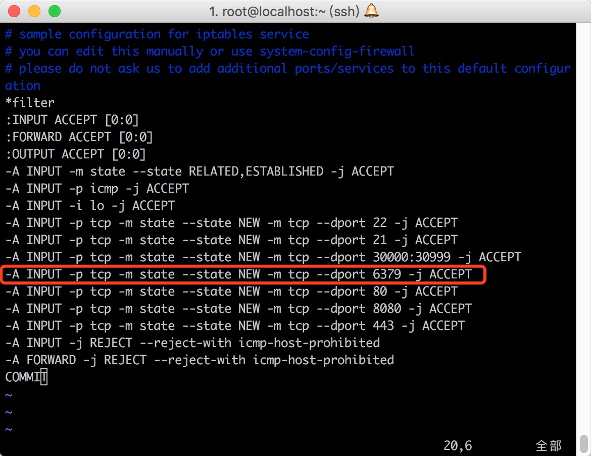
The rest is firewall configuration. Port 6379 needs to be added to the firewall whitelist. The host is using iptables

vim /etc/sysconfig/iptables

Add: -a Input-P TCP-M State — State new-m TCP — Dport 6379-j ACCEPT as shown in the figure below:

About the iptables and firewall configuration, please see this article: http://blog.csdn.net/XIANZHIXIANZHIXIAN/article/details/78918772
So let’s start Redis

redis-server /usr/local/redis-4.0.7/redis.conf

Check whether the Redis process has been started successfully. For example, the plan has been started successfully:
ps -ef | grep redis

Test the Java code after successful startup

package com.yufeng.redis.demo;

import redis.clients.jedis.Jedis;
import redis.clients.jedis.JedisPool;

/**
 * Monitoring Data in Redis
 */
public class ShowRedis implements Runnable{

    JedisPool jedisPool=new JedisPool("192.168.56.101",6379);
    Jedis jedis=null;
    public void run() {
        while(true){

            try{
                jedis=jedisPool.getResource();
                System.out.println(jedis.lrange("runningtask",0L,99L));
                jedis.close();
                Thread.sleep(5000L);
            }catch (Exception e){
                e.printStackTrace();
            }
        }
    }
}

The Main function of the

package com.yufeng.redis.demo;

import redis.clients.jedis.Jedis;

/**
 * Redis Test Code
 */
public class Main {

    public static void main(String[] args){
        try {

            Thread spyer = new Thread(new ShowRedis());
            spyer.start();
            //Main thread hibernation
            Thread.sleep(Long.MAX_VALUE);
        }catch (Exception e){
            e.printStackTrace();
        }
    }
}

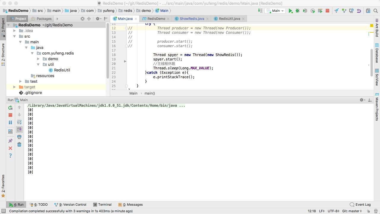
The result is shown in the figure. Since there is no data in the runningTask queue of the building owner, the value obtained by LLen () is 0. Congratulations, your Redis configuration and installation is complete!

Then talk about the pit, here used gay purple, said these pits made the landlord like the sun as uncomfortable as a; Avoid wasting your time and energy in these pits!
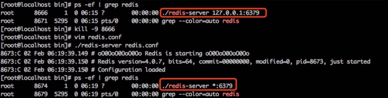
First, ps-ef | grep Java shows that the Redis process is started, but cannot be accessed by an out-of-network application

Compare the two red boxes in the figure, the first one is./ redIS-Server 127.0.0.1:6379, the second one is./ Redis-Server 127.0.0.0.1:6379; This is because the bind 127.0.0.1 in the redis.conf configuration is not commented out, so restart the Redis service!
Second, bind 127.0.0.1 cannot be connected in the program after it has been commented out

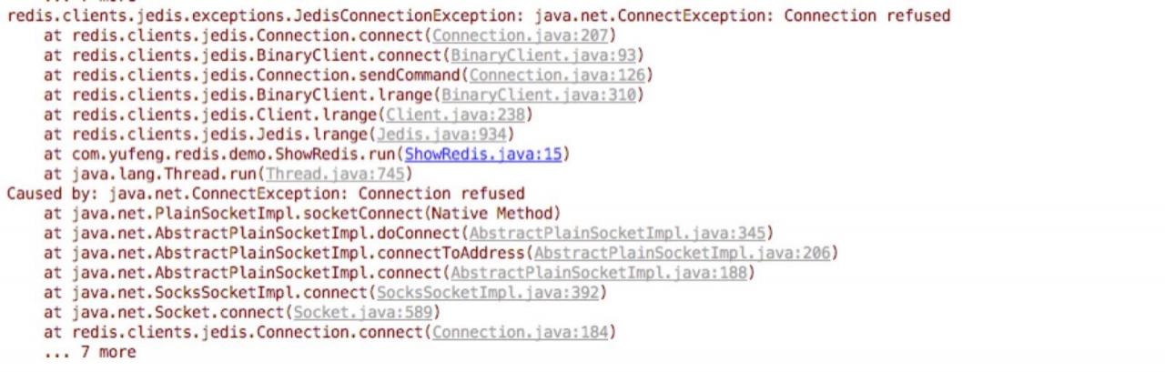
M: Connection union, refused. There are two possible reasons:
1. Redis has the protected-mode or yes status, and is not set to the protected-mode no
2, then is the firewall ah, firewall ah, firewall ah!! Remember to open port 6379 in the firewall!!
Redis. Conf configuration file

# Redis configuration file example.
#
# Note that in order to read the configuration file, Redis must be
# started with the file path as first argument:
#
# ./redis-server /path/to/redis.conf

# Note on units: when memory size is needed, it is possible to specify
# it in the usual form of 1k 5GB 4M and so forth:
#
# 1k => 1000 bytes
# 1kb => 1024 bytes
# 1m => 1000000 bytes
# 1mb => 1024*1024 bytes
# 1g => 1000000000 bytes
# 1gb => 1024*1024*1024 bytes
#
# units are case insensitive so 1GB 1Gb 1gB are all the same.

################################## INCLUDES ###################################

# Include one or more other config files here.  This is useful if you
# have a standard template that goes to all Redis servers but also need
# to customize a few per-server settings.  Include files can include
# other files, so use this wisely.
#
# Notice option "include" won't be rewritten by command "CONFIG REWRITE"
# from admin or Redis Sentinel. Since Redis always uses the last processed
# line as value of a configuration directive, you'd better put includes
# at the beginning of this file to avoid overwriting config change at runtime.
#
# If instead you are interested in using includes to override configuration
# options, it is better to use include as the last line.
#
# include /path/to/local.conf
# include /path/to/other.conf

################################## MODULES #####################################

# Load modules at startup. If the server is not able to load modules
# it will abort. It is possible to use multiple loadmodule directives.
#
# loadmodule /path/to/my_module.so
# loadmodule /path/to/other_module.so

################################## NETWORK #####################################

# By default, if no "bind" configuration directive is specified, Redis listens
# for connections from all the network interfaces available on the server.
# It is possible to listen to just one or multiple selected interfaces using
# the "bind" configuration directive, followed by one or more IP addresses.
#
# Examples:
#
# bind 192.168.1.100 10.0.0.1
# bind 127.0.0.1 ::1
#
# ~~~ WARNING ~~~ If the computer running Redis is directly exposed to the
# internet, binding to all the interfaces is dangerous and will expose the
# instance to everybody on the internet. So by default we uncomment the
# following bind directive, that will force Redis to listen only into
# the IPv4 lookback interface address (this means Redis will be able to
# accept connections only from clients running into the same computer it
# is running).
#
# IF YOU ARE SURE YOU WANT YOUR INSTANCE TO LISTEN TO ALL THE INTERFACES
# JUST COMMENT THE FOLLOWING LINE.
# ~~~~~~~~~~~~~~~~~~~~~~~~~~~~~~~~~~~~~~~~~~~~~~~~~~~~~~~~~~~~~~~~~~~~~~~~
#bind 127.0.0.1

# Protected mode is a layer of security protection, in order to avoid that
# Redis instances left open on the internet are accessed and exploited.
#
# When protected mode is on and if:
#
# 1) The server is not binding explicitly to a set of addresses using the
#    "bind" directive.
# 2) No password is configured.
#
# The server only accepts connections from clients connecting from the
# IPv4 and IPv6 loopback addresses 127.0.0.1 and ::1, and from Unix domain
# sockets.
#
# By default protected mode is enabled. You should disable it only if
# you are sure you want clients from other hosts to connect to Redis
# even if no authentication is configured, nor a specific set of interfaces
# are explicitly listed using the "bind" directive.
protected-mode no 

# Accept connections on the specified port, default is 6379 (IANA #815344).
# If port 0 is specified Redis will not listen on a TCP socket.
port 6379

# TCP listen() backlog.
#
# In high requests-per-second environments you need an high backlog in order
# to avoid slow clients connections issues. Note that the Linux kernel
# will silently truncate it to the value of /proc/sys/net/core/somaxconn so
# make sure to raise both the value of somaxconn and tcp_max_syn_backlog
# in order to get the desired effect.
tcp-backlog 511

# Unix socket.
#
# Specify the path for the Unix socket that will be used to listen for
# incoming connections. There is no default, so Redis will not listen
# on a unix socket when not specified.
#
# unixsocket /tmp/redis.sock
# unixsocketperm 700

# Close the connection after a client is idle for N seconds (0 to disable)
timeout 0

# TCP keepalive.
#
# If non-zero, use SO_KEEPALIVE to send TCP ACKs to clients in absence
# of communication. This is useful for two reasons:

# 1) Detect dead peers.
# 2) Take the connection alive from the point of view of network
#    equipment in the middle.
#
# On Linux, the specified value (in seconds) is the period used to send ACKs.
# Note that to close the connection the double of the time is needed.
# On other kernels the period depends on the kernel configuration.
#
# A reasonable value for this option is 300 seconds, which is the new
# Redis default starting with Redis 3.2.1.
tcp-keepalive 300

################################# GENERAL #####################################

# By default Redis does not run as a daemon. Use 'yes' if you need it.
# Note that Redis will write a pid file in /var/run/redis.pid when daemonized.
daemonize yes

# If you run Redis from upstart or systemd, Redis can interact with your
# supervision tree. Options:
#   supervised no      - no supervision interaction
#   supervised upstart - signal upstart by putting Redis into SIGSTOP mode
#   supervised systemd - signal systemd by writing READY=1 to $NOTIFY_SOCKET
#   supervised auto    - detect upstart or systemd method based on
#                        UPSTART_JOB or NOTIFY_SOCKET environment variables
# Note: these supervision methods only signal "process is ready."
#       They do not enable continuous liveness pings back to your supervisor.
supervised no

# If a pid file is specified, Redis writes it where specified at startup
# and removes it at exit.
#
# When the server runs non daemonized, no pid file is created if none is
# specified in the configuration. When the server is daemonized, the pid file
# is used even if not specified, defaulting to "/var/run/redis.pid".
#
# Creating a pid file is best effort: if Redis is not able to create it
# nothing bad happens, the server will start and run normally.
pidfile /var/run/redis_6379.pid

# Specify the server verbosity level.
# This can be one of:
# debug (a lot of information, useful for development/testing)
# verbose (many rarely useful info, but not a mess like the debug level)
# notice (moderately verbose, what you want in production probably)
# warning (only very important/critical messages are logged)
loglevel notice

# Specify the log file name. Also the empty string can be used to force
# Redis to log on the standard output. Note that if you use standard
# output for logging but daemonize, logs will be sent to /dev/null
logfile ""

# To enable logging to the system logger, just set 'syslog-enabled' to yes,
# and optionally update the other syslog parameters to suit your needs.
# syslog-enabled no

# Specify the syslog identity.
# syslog-ident redis

# Specify the syslog facility. Must be USER or between LOCAL0-LOCAL7.
# syslog-facility local0

# Set the number of databases. The default database is DB 0, you can select
# a different one on a per-connection basis using SELECT <dbid> where
# dbid is a number between 0 and 'databases'-1
databases 16

# By default Redis shows an ASCII art logo only when started to log to the
# standard output and if the standard output is a TTY. Basically this means
# that normally a logo is displayed only in interactive sessions.
#
# However it is possible to force the pre-4.0 behavior and always show a
# ASCII art logo in startup logs by setting the following option to yes.
always-show-logo yes

################################ SNAPSHOTTING  ################################
#
# Save the DB on disk:
#
#   save <seconds> <changes>
#
#   Will save the DB if both the given number of seconds and the given
#   number of write operations against the DB occurred.
#
#   In the example below the behaviour will be to save:
#   after 900 sec (15 min) if at least 1 key changed
#   after 300 sec (5 min) if at least 10 keys changed
#   after 60 sec if at least 10000 keys changed
#
#   Note: you can disable saving completely by commenting out all "save" lines.
#
#   It is also possible to remove all the previously configured save
#   points by adding a save directive with a single empty string argument
#   like in the following example:
#
#   save ""

save 900 1
save 300 10
save 60 10000

# By default Redis will stop accepting writes if RDB snapshots are enabled
# (at least one save point) and the latest background save failed.
# This will make the user aware (in a hard way) that data is not persisting
# on disk properly, otherwise chances are that no one will notice and some
# disaster will happen.
#
# If the background saving process will start working again Redis will
# automatically allow writes again.
#
# However if you have setup your proper monitoring of the Redis server
# and persistence, you may want to disable this feature so that Redis will
# continue to work as usual even if there are problems with disk,
# permissions, and so forth.
stop-writes-on-bgsave-error yes

# Compress string objects using LZF when dump .rdb databases?
# For default that's set to 'yes' as it's almost always a win.
# If you want to save some CPU in the saving child set it to 'no' but
# the dataset will likely be bigger if you have compressible values or keys.
rdbcompression yes

# Since version 5 of RDB a CRC64 checksum is placed at the end of the file.
# This makes the format more resistant to corruption but there is a performance
# hit to pay (around 10%) when saving and loading RDB files, so you can disable it
# for maximum performances.
#
# RDB files created with checksum disabled have a checksum of zero that will
# tell the loading code to skip the check.
rdbchecksum yes

# The filename where to dump the DB
dbfilename dump.rdb

# The working directory.
#
# The DB will be written inside this directory, with the filename specified
# above using the 'dbfilename' configuration directive.
#
# The Append Only File will also be created inside this directory.
#
# Note that you must specify a directory here, not a file name.
dir ./

################################# REPLICATION #################################

# Master-Slave replication. Use slaveof to make a Redis instance a copy of
# another Redis server. A few things to understand ASAP about Redis replication.
#
# 1) Redis replication is asynchronous, but you can configure a master to
#    stop accepting writes if it appears to be not connected with at least
#    a given number of slaves.
# 2) Redis slaves are able to perform a partial resynchronization with the
#    master if the replication link is lost for a relatively small amount of
#    time. You may want to configure the replication backlog size (see the next
#    sections of this file) with a sensible value depending on your needs.
# 3) Replication is automatic and does not need user intervention. After a
#    network partition slaves automatically try to reconnect to masters
#    and resynchronize with them.
#
# slaveof <masterip> <masterport>

# If the master is password protected (using the "requirepass" configuration
# directive below) it is possible to tell the slave to authenticate before
# starting the replication synchronization process, otherwise the master will
# refuse the slave request.
#
# masterauth <master-password>

# When a slave loses its connection with the master, or when the replication
# is still in progress, the slave can act in two different ways:
#
# 1) if slave-serve-stale-data is set to 'yes' (the default) the slave will
#    still reply to client requests, possibly with out of date data, or the
#    data set may just be empty if this is the first synchronization.
#
# 2) if slave-serve-stale-data is set to 'no' the slave will reply with
#    an error "SYNC with master in progress" to all the kind of commands
#    but to INFO and SLAVEOF.
#
slave-serve-stale-data yes

# You can configure a slave instance to accept writes or not. Writing against
# a slave instance may be useful to store some ephemeral data (because data
# written on a slave will be easily deleted after resync with the master) but
# may also cause problems if clients are writing to it because of a
# misconfiguration.
#
# Since Redis 2.6 by default slaves are read-only.
#
# Note: read only slaves are not designed to be exposed to untrusted clients
# on the internet. It's just a protection layer against misuse of the instance.
# Still a read only slave exports by default all the administrative commands
# such as CONFIG, DEBUG, and so forth. To a limited extent you can improve
# security of read only slaves using 'rename-command' to shadow all the
# administrative/dangerous commands.
slave-read-only yes

# Replication SYNC strategy: disk or socket.
#
# -------------------------------------------------------
# WARNING: DISKLESS REPLICATION IS EXPERIMENTAL CURRENTLY
# -------------------------------------------------------
#
# New slaves and reconnecting slaves that are not able to continue the replication
# process just receiving differences, need to do what is called a "full
# synchronization". An RDB file is transmitted from the master to the slaves.
# The transmission can happen in two different ways:
#
# 1) Disk-backed: The Redis master creates a new process that writes the RDB
#                 file on disk. Later the file is transferred by the parent
#                 process to the slaves incrementally.
# 2) Diskless: The Redis master creates a new process that directly writes the
#              RDB file to slave sockets, without touching the disk at all.
#
# With disk-backed replication, while the RDB file is generated, more slaves
# can be queued and served with the RDB file as soon as the current child producing
# the RDB file finishes its work. With diskless replication instead once
# the transfer starts, new slaves arriving will be queued and a new transfer
# will start when the current one terminates.
#
# When diskless replication is used, the master waits a configurable amount of
# time (in seconds) before starting the transfer in the hope that multiple slaves
# will arrive and the transfer can be parallelized.
#
# With slow disks and fast (large bandwidth) networks, diskless replication
# works better.
repl-diskless-sync no

# When diskless replication is enabled, it is possible to configure the delay
# the server waits in order to spawn the child that transfers the RDB via socket
# to the slaves.
#
# This is important since once the transfer starts, it is not possible to serve
# new slaves arriving, that will be queued for the next RDB transfer, so the server
# waits a delay in order to let more slaves arrive.
#
# The delay is specified in seconds, and by default is 5 seconds. To disable
# it entirely just set it to 0 seconds and the transfer will start ASAP.
repl-diskless-sync-delay 5

# Slaves send PINGs to server in a predefined interval. It's possible to change
# this interval with the repl_ping_slave_period option. The default value is 10
# seconds.
#
# repl-ping-slave-period 10

# The following option sets the replication timeout for:
#
# 1) Bulk transfer I/O during SYNC, from the point of view of slave.
# 2) Master timeout from the point of view of slaves (data, pings).
# 3) Slave timeout from the point of view of masters (REPLCONF ACK pings).
#
# It is important to make sure that this value is greater than the value
# specified for repl-ping-slave-period otherwise a timeout will be detected
# every time there is low traffic between the master and the slave.
#
# repl-timeout 60

# Disable TCP_NODELAY on the slave socket after SYNC?
#
# If you select "yes" Redis will use a smaller number of TCP packets and
# less bandwidth to send data to slaves. But this can add a delay for
# the data to appear on the slave side, up to 40 milliseconds with
# Linux kernels using a default configuration.
#
# If you select "no" the delay for data to appear on the slave side will
# be reduced but more bandwidth will be used for replication.
#
# By default we optimize for low latency, but in very high traffic conditions
# or when the master and slaves are many hops away, turning this to "yes" may
# be a good idea.
repl-disable-tcp-nodelay no

# Set the replication backlog size. The backlog is a buffer that accumulates
# slave data when slaves are disconnected for some time, so that when a slave
# wants to reconnect again, often a full resync is not needed, but a partial
# resync is enough, just passing the portion of data the slave missed while
# disconnected.
#
# The bigger the replication backlog, the longer the time the slave can be
# disconnected and later be able to perform a partial resynchronization.
#
# The backlog is only allocated once there is at least a slave connected.
#
# repl-backlog-size 1mb

# After a master has no longer connected slaves for some time, the backlog
# will be freed. The following option configures the amount of seconds that
# need to elapse, starting from the time the last slave disconnected, for
# the backlog buffer to be freed.
#
# Note that slaves never free the backlog for timeout, since they may be
# promoted to masters later, and should be able to correctly "partially
# resynchronize" with the slaves: hence they should always accumulate backlog.
#
# A value of 0 means to never release the backlog.
#
# repl-backlog-ttl 3600

# The slave priority is an integer number published by Redis in the INFO output.
# It is used by Redis Sentinel in order to select a slave to promote into a
# master if the master is no longer working correctly.
#
# A slave with a low priority number is considered better for promotion, so
# for instance if there are three slaves with priority 10, 100, 25 Sentinel will
# pick the one with priority 10, that is the lowest.
#
# However a special priority of 0 marks the slave as not able to perform the
# role of master, so a slave with priority of 0 will never be selected by
# Redis Sentinel for promotion.
#
# By default the priority is 100.
slave-priority 100

# It is possible for a master to stop accepting writes if there are less than
# N slaves connected, having a lag less or equal than M seconds.
#
# The N slaves need to be in "online" state.
#
# The lag in seconds, that must be <= the specified value, is calculated from
# the last ping received from the slave, that is usually sent every second.
#
# This option does not GUARANTEE that N replicas will accept the write, but
# will limit the window of exposure for lost writes in case not enough slaves
# are available, to the specified number of seconds.
#
# For example to require at least 3 slaves with a lag <= 10 seconds use:
#
# min-slaves-to-write 3
# min-slaves-max-lag 10
#
# Setting one or the other to 0 disables the feature.
#
# By default min-slaves-to-write is set to 0 (feature disabled) and
# min-slaves-max-lag is set to 10.

# A Redis master is able to list the address and port of the attached
# slaves in different ways. For example the "INFO replication" section
# offers this information, which is used, among other tools, by
# Redis Sentinel in order to discover slave instances.
# Another place where this info is available is in the output of the
# "ROLE" command of a master.
#
# The listed IP and address normally reported by a slave is obtained
# in the following way:
#
#   IP: The address is auto detected by checking the peer address
#   of the socket used by the slave to connect with the master.
#
#   Port: The port is communicated by the slave during the replication
#   handshake, and is normally the port that the slave is using to
#   list for connections.
#
# However when port forwarding or Network Address Translation (NAT) is
# used, the slave may be actually reachable via different IP and port
# pairs. The following two options can be used by a slave in order to
# report to its master a specific set of IP and port, so that both INFO
# and ROLE will report those values.
#
# There is no need to use both the options if you need to override just
# the port or the IP address.
#
# slave-announce-ip 5.5.5.5
# slave-announce-port 1234

################################## SECURITY ###################################

# Require clients to issue AUTH <PASSWORD> before processing any other
# commands.  This might be useful in environments in which you do not trust
# others with access to the host running redis-server.
#
# This should stay commented out for backward compatibility and because most
# people do not need auth (e.g. they run their own servers).
#
# Warning: since Redis is pretty fast an outside user can try up to
# 150k passwords per second against a good box. This means that you should
# use a very strong password otherwise it will be very easy to break.
#
# requirepass foobared

# Command renaming.
#
# It is possible to change the name of dangerous commands in a shared
# environment. For instance the CONFIG command may be renamed into something
# hard to guess so that it will still be available for internal-use tools
# but not available for general clients.
#
# Example:
#
# rename-command CONFIG b840fc02d524045429941cc15f59e41cb7be6c52
#
# It is also possible to completely kill a command by renaming it into
# an empty string:
#
# rename-command CONFIG ""
#
# Please note that changing the name of commands that are logged into the
# AOF file or transmitted to slaves may cause problems.

################################### CLIENTS ####################################

# Set the max number of connected clients at the same time. By default
# this limit is set to 10000 clients, however if the Redis server is not
# able to configure the process file limit to allow for the specified limit
# the max number of allowed clients is set to the current file limit
# minus 32 (as Redis reserves a few file descriptors for internal uses).
#
# Once the limit is reached Redis will close all the new connections sending
# an error 'max number of clients reached'.
#
# maxclients 10000

############################## MEMORY MANAGEMENT ################################

# Set a memory usage limit to the specified amount of bytes.
# When the memory limit is reached Redis will try to remove keys
# according to the eviction policy selected (see maxmemory-policy).
#
# If Redis can't remove keys according to the policy, or if the policy is
# set to 'noeviction', Redis will start to reply with errors to commands
# that would use more memory, like SET, LPUSH, and so on, and will continue
# to reply to read-only commands like GET.
#
# This option is usually useful when using Redis as an LRU or LFU cache, or to
# set a hard memory limit for an instance (using the 'noeviction' policy).
#
# WARNING: If you have slaves attached to an instance with maxmemory on,
# the size of the output buffers needed to feed the slaves are subtracted
# from the used memory count, so that network problems/resyncs will
# not trigger a loop where keys are evicted, and in turn the output
# buffer of slaves is full with DELs of keys evicted triggering the deletion
# of more keys, and so forth until the database is completely emptied.
#
# In short... if you have slaves attached it is suggested that you set a lower
# limit for maxmemory so that there is some free RAM on the system for slave
# output buffers (but this is not needed if the policy is 'noeviction').
#
# maxmemory <bytes>

# MAXMEMORY POLICY: how Redis will select what to remove when maxmemory
# is reached. You can select among five behaviors:
#
# volatile-lru -> Evict using approximated LRU among the keys with an expire set.
# allkeys-lru -> Evict any key using approximated LRU.
# volatile-lfu -> Evict using approximated LFU among the keys with an expire set.
# allkeys-lfu -> Evict any key using approximated LFU.
# volatile-random -> Remove a random key among the ones with an expire set.
# allkeys-random -> Remove a random key, any key.
# volatile-ttl -> Remove the key with the nearest expire time (minor TTL)
# noeviction -> Don't evict anything, just return an error on write operations.
#
# LRU means Least Recently Used
# LFU means Least Frequently Used
#
# Both LRU, LFU and volatile-ttl are implemented using approximated
# randomized algorithms.
#
# Note: with any of the above policies, Redis will return an error on write
#       operations, when there are no suitable keys for eviction.
#
#       At the date of writing these commands are: set setnx setex append
#       incr decr rpush lpush rpushx lpushx linsert lset rpoplpush sadd
#       sinter sinterstore sunion sunionstore sdiff sdiffstore zadd zincrby
#       zunionstore zinterstore hset hsetnx hmset hincrby incrby decrby
#       getset mset msetnx exec sort
#
# The default is:
#
# maxmemory-policy noeviction

# LRU, LFU and minimal TTL algorithms are not precise algorithms but approximated
# algorithms (in order to save memory), so you can tune it for speed or
# accuracy. For default Redis will check five keys and pick the one that was
# used less recently, you can change the sample size using the following
# configuration directive.
#
# The default of 5 produces good enough results. 10 Approximates very closely
# true LRU but costs more CPU. 3 is faster but not very accurate.
#
# maxmemory-samples 5

############################# LAZY FREEING ####################################

# Redis has two primitives to delete keys. One is called DEL and is a blocking
# deletion of the object. It means that the server stops processing new commands
# in order to reclaim all the memory associated with an object in a synchronous
# way. If the key deleted is associated with a small object, the time needed
# in order to execute the DEL command is very small and comparable to most other
# O(1) or O(log_N) commands in Redis. However if the key is associated with an
# aggregated value containing millions of elements, the server can block for
# a long time (even seconds) in order to complete the operation.
#
# For the above reasons Redis also offers non blocking deletion primitives
# such as UNLINK (non blocking DEL) and the ASYNC option of FLUSHALL and
# FLUSHDB commands, in order to reclaim memory in background. Those commands
# are executed in constant time. Another thread will incrementally free the
# object in the background as fast as possible.
#
# DEL, UNLINK and ASYNC option of FLUSHALL and FLUSHDB are user-controlled.
# It's up to the design of the application to understand when it is a good
# idea to use one or the other. However the Redis server sometimes has to
# delete keys or flush the whole database as a side effect of other operations.
# Specifically Redis deletes objects independently of a user call in the
# following scenarios:
#
# 1) On eviction, because of the maxmemory and maxmemory policy configurations,
#    in order to make room for new data, without going over the specified
#    memory limit.
# 2) Because of expire: when a key with an associated time to live (see the
#    EXPIRE command) must be deleted from memory.
# 3) Because of a side effect of a command that stores data on a key that may
#    already exist. For example the RENAME command may delete the old key
#    content when it is replaced with another one. Similarly SUNIONSTORE
#    or SORT with STORE option may delete existing keys. The SET command
#    itself removes any old content of the specified key in order to replace
#    it with the specified string.
# 4) During replication, when a slave performs a full resynchronization with
#    its master, the content of the whole database is removed in order to
#    load the RDB file just transfered.
#
# In all the above cases the default is to delete objects in a blocking way,
# like if DEL was called. However you can configure each case specifically
# in order to instead release memory in a non-blocking way like if UNLINK
# was called, using the following configuration directives:

lazyfree-lazy-eviction no
lazyfree-lazy-expire no
lazyfree-lazy-server-del no
slave-lazy-flush no

############################## APPEND ONLY MODE ###############################

# By default Redis asynchronously dumps the dataset on disk. This mode is
# good enough in many applications, but an issue with the Redis process or
# a power outage may result into a few minutes of writes lost (depending on
# the configured save points).
#
# The Append Only File is an alternative persistence mode that provides
# much better durability. For instance using the default data fsync policy
# (see later in the config file) Redis can lose just one second of writes in a
# dramatic event like a server power outage, or a single write if something
# wrong with the Redis process itself happens, but the operating system is
# still running correctly.
#
# AOF and RDB persistence can be enabled at the same time without problems.
# If the AOF is enabled on startup Redis will load the AOF, that is the file
# with the better durability guarantees.
#
# Please check http://redis.io/topics/persistence for more information.

appendonly no

# The name of the append only file (default: "appendonly.aof")

appendfilename "appendonly.aof"

# The fsync() call tells the Operating System to actually write data on disk
# instead of waiting for more data in the output buffer. Some OS will really flush
# data on disk, some other OS will just try to do it ASAP.
#
# Redis supports three different modes:
#
# no: don't fsync, just let the OS flush the data when it wants. Faster.
# always: fsync after every write to the append only log. Slow, Safest.
# everysec: fsync only one time every second. Compromise.
#
# The default is "everysec", as that's usually the right compromise between
# speed and data safety. It's up to you to understand if you can relax this to
# "no" that will let the operating system flush the output buffer when
# it wants, for better performances (but if you can live with the idea of
# some data loss consider the default persistence mode that's snapshotting),
# or on the contrary, use "always" that's very slow but a bit safer than
# everysec.
#
# More details please check the following article:
# http://antirez.com/post/redis-persistence-demystified.html
#
# If unsure, use "everysec".

# appendfsync always
appendfsync everysec
# appendfsync no

# When the AOF fsync policy is set to always or everysec, and a background
# saving process (a background save or AOF log background rewriting) is
# performing a lot of I/O against the disk, in some Linux configurations
# Redis may block too long on the fsync() call. Note that there is no fix for
# this currently, as even performing fsync in a different thread will block
# our synchronous write(2) call.
#
# In order to mitigate this problem it's possible to use the following option
# that will prevent fsync() from being called in the main process while a
# BGSAVE or BGREWRITEAOF is in progress.
#
# This means that while another child is saving, the durability of Redis is
# the same as "appendfsync none". In practical terms, this means that it is
# possible to lose up to 30 seconds of log in the worst scenario (with the
# default Linux settings).
#
# If you have latency problems turn this to "yes". Otherwise leave it as
# "no" that is the safest pick from the point of view of durability.

no-appendfsync-on-rewrite no

# Automatic rewrite of the append only file.
# Redis is able to automatically rewrite the log file implicitly calling
# BGREWRITEAOF when the AOF log size grows by the specified percentage.
#
# This is how it works: Redis remembers the size of the AOF file after the
# latest rewrite (if no rewrite has happened since the restart, the size of
# the AOF at startup is used).
#
# This base size is compared to the current size. If the current size is
# bigger than the specified percentage, the rewrite is triggered. Also
# you need to specify a minimal size for the AOF file to be rewritten, this
# is useful to avoid rewriting the AOF file even if the percentage increase
# is reached but it is still pretty small.
#
# Specify a percentage of zero in order to disable the automatic AOF
# rewrite feature.

auto-aof-rewrite-percentage 100
auto-aof-rewrite-min-size 64mb

# An AOF file may be found to be truncated at the end during the Redis
# startup process, when the AOF data gets loaded back into memory.
# This may happen when the system where Redis is running
# crashes, especially when an ext4 filesystem is mounted without the
# data=ordered option (however this can't happen when Redis itself
# crashes or aborts but the operating system still works correctly).
#
# Redis can either exit with an error when this happens, or load as much
# data as possible (the default now) and start if the AOF file is found
# to be truncated at the end. The following option controls this behavior.
#
# If aof-load-truncated is set to yes, a truncated AOF file is loaded and
# the Redis server starts emitting a log to inform the user of the event.
# Otherwise if the option is set to no, the server aborts with an error
# and refuses to start. When the option is set to no, the user requires
# to fix the AOF file using the "redis-check-aof" utility before to restart
# the server.
#
# Note that if the AOF file will be found to be corrupted in the middle
# the server will still exit with an error. This option only applies when
# Redis will try to read more data from the AOF file but not enough bytes
# will be found.
aof-load-truncated yes

# When rewriting the AOF file, Redis is able to use an RDB preamble in the
# AOF file for faster rewrites and recoveries. When this option is turned
# on the rewritten AOF file is composed of two different stanzas:
#
#   [RDB file][AOF tail]
#
# When loading Redis recognizes that the AOF file starts with the "REDIS"
# string and loads the prefixed RDB file, and continues loading the AOF
# tail.
#
# This is currently turned off by default in order to avoid the surprise
# of a format change, but will at some point be used as the default.
aof-use-rdb-preamble no

################################ LUA SCRIPTING  ###############################

# Max execution time of a Lua script in milliseconds.
#
# If the maximum execution time is reached Redis will log that a script is
# still in execution after the maximum allowed time and will start to
# reply to queries with an error.
#
# When a long running script exceeds the maximum execution time only the
# SCRIPT KILL and SHUTDOWN NOSAVE commands are available. The first can be
# used to stop a script that did not yet called write commands. The second
# is the only way to shut down the server in the case a write command was
# already issued by the script but the user doesn't want to wait for the natural
# termination of the script.
#
# Set it to 0 or a negative value for unlimited execution without warnings.
lua-time-limit 5000

################################ REDIS CLUSTER  ###############################
#
# ++++++++++++++++++++++++++++++++++++++++++++++++++++++++++++++++++++++++++++
# WARNING EXPERIMENTAL: Redis Cluster is considered to be stable code, however
# in order to mark it as "mature" we need to wait for a non trivial percentage
# of users to deploy it in production.
# ++++++++++++++++++++++++++++++++++++++++++++++++++++++++++++++++++++++++++++
#
# Normal Redis instances can't be part of a Redis Cluster; only nodes that are
# started as cluster nodes can. In order to start a Redis instance as a
# cluster node enable the cluster support uncommenting the following:
#
# cluster-enabled yes

# Every cluster node has a cluster configuration file. This file is not
# intended to be edited by hand. It is created and updated by Redis nodes.
# Every Redis Cluster node requires a different cluster configuration file.
# Make sure that instances running in the same system do not have
# overlapping cluster configuration file names.
#
# cluster-config-file nodes-6379.conf

# Cluster node timeout is the amount of milliseconds a node must be unreachable
# for it to be considered in failure state.
# Most other internal time limits are multiple of the node timeout.
#
# cluster-node-timeout 15000

# A slave of a failing master will avoid to start a failover if its data
# looks too old.
#
# There is no simple way for a slave to actually have an exact measure of
# its "data age", so the following two checks are performed:
#
# 1) If there are multiple slaves able to failover, they exchange messages
#    in order to try to give an advantage to the slave with the best
#    replication offset (more data from the master processed).
#    Slaves will try to get their rank by offset, and apply to the start
#    of the failover a delay proportional to their rank.
#
# 2) Every single slave computes the time of the last interaction with
#    its master. This can be the last ping or command received (if the master
#    is still in the "connected" state), or the time that elapsed since the
#    disconnection with the master (if the replication link is currently down).
#    If the last interaction is too old, the slave will not try to failover
#    at all.
#
# The point "2" can be tuned by user. Specifically a slave will not perform
# the failover if, since the last interaction with the master, the time
# elapsed is greater than:
#
#   (node-timeout * slave-validity-factor) + repl-ping-slave-period
#
# So for example if node-timeout is 30 seconds, and the slave-validity-factor
# is 10, and assuming a default repl-ping-slave-period of 10 seconds, the
# slave will not try to failover if it was not able to talk with the master
# for longer than 310 seconds.
#
# A large slave-validity-factor may allow slaves with too old data to failover
# a master, while a too small value may prevent the cluster from being able to
# elect a slave at all.
#
# For maximum availability, it is possible to set the slave-validity-factor
# to a value of 0, which means, that slaves will always try to failover the
# master regardless of the last time they interacted with the master.
# (However they'll always try to apply a delay proportional to their
# offset rank).
#
# Zero is the only value able to guarantee that when all the partitions heal
# the cluster will always be able to continue.
#
# cluster-slave-validity-factor 10

# Cluster slaves are able to migrate to orphaned masters, that are masters
# that are left without working slaves. This improves the cluster ability
# to resist to failures as otherwise an orphaned master can't be failed over
# in case of failure if it has no working slaves.
#
# Slaves migrate to orphaned masters only if there are still at least a
# given number of other working slaves for their old master. This number
# is the "migration barrier". A migration barrier of 1 means that a slave
# will migrate only if there is at least 1 other working slave for its master
# and so forth. It usually reflects the number of slaves you want for every
# master in your cluster.
#
# Default is 1 (slaves migrate only if their masters remain with at least
# one slave). To disable migration just set it to a very large value.
# A value of 0 can be set but is useful only for debugging and dangerous
# in production.
#
# cluster-migration-barrier 1

# By default Redis Cluster nodes stop accepting queries if they detect there
# is at least an hash slot uncovered (no available node is serving it).
# This way if the cluster is partially down (for example a range of hash slots
# are no longer covered) all the cluster becomes, eventually, unavailable.
# It automatically returns available as soon as all the slots are covered again.
#
# However sometimes you want the subset of the cluster which is working,
# to continue to accept queries for the part of the key space that is still
# covered. In order to do so, just set the cluster-require-full-coverage
# option to no.
#
# cluster-require-full-coverage yes

# In order to setup your cluster make sure to read the documentation
# available at http://redis.io web site.

########################## CLUSTER DOCKER/NAT support  ########################

# In certain deployments, Redis Cluster nodes address discovery fails, because
# addresses are NAT-ted or because ports are forwarded (the typical case is
# Docker and other containers).
#
# In order to make Redis Cluster working in such environments, a static
# configuration where each node knows its public address is needed. The
# following two options are used for this scope, and are:
#
# * cluster-announce-ip
# * cluster-announce-port
# * cluster-announce-bus-port
#
# Each instruct the node about its address, client port, and cluster message
# bus port. The information is then published in the header of the bus packets
# so that other nodes will be able to correctly map the address of the node
# publishing the information.
#
# If the above options are not used, the normal Redis Cluster auto-detection
# will be used instead.
#
# Note that when remapped, the bus port may not be at the fixed offset of
# clients port + 10000, so you can specify any port and bus-port depending
# on how they get remapped. If the bus-port is not set, a fixed offset of
# 10000 will be used as usually.
#
# Example:
#
# cluster-announce-ip 10.1.1.5
# cluster-announce-port 6379
# cluster-announce-bus-port 6380

################################## SLOW LOG ###################################

# The Redis Slow Log is a system to log queries that exceeded a specified
# execution time. The execution time does not include the I/O operations
# like talking with the client, sending the reply and so forth,
# but just the time needed to actually execute the command (this is the only
# stage of command execution where the thread is blocked and can not serve
# other requests in the meantime).
#
# You can configure the slow log with two parameters: one tells Redis
# what is the execution time, in microseconds, to exceed in order for the
# command to get logged, and the other parameter is the length of the
# slow log. When a new command is logged the oldest one is removed from the
# queue of logged commands.

# The following time is expressed in microseconds, so 1000000 is equivalent
# to one second. Note that a negative number disables the slow log, while
# a value of zero forces the logging of every command.
slowlog-log-slower-than 10000

# There is no limit to this length. Just be aware that it will consume memory.
# You can reclaim memory used by the slow log with SLOWLOG RESET.
slowlog-max-len 128

################################ LATENCY MONITOR ##############################

# The Redis latency monitoring subsystem samples different operations
# at runtime in order to collect data related to possible sources of
# latency of a Redis instance.
#
# Via the LATENCY command this information is available to the user that can
# print graphs and obtain reports.
#
# The system only logs operations that were performed in a time equal or
# greater than the amount of milliseconds specified via the
# latency-monitor-threshold configuration directive. When its value is set
# to zero, the latency monitor is turned off.
#
# By default latency monitoring is disabled since it is mostly not needed
# if you don't have latency issues, and collecting data has a performance
# impact, that while very small, can be measured under big load. Latency
# monitoring can easily be enabled at runtime using the command
# "CONFIG SET latency-monitor-threshold <milliseconds>" if needed.
latency-monitor-threshold 0

############################# EVENT NOTIFICATION ##############################

# Redis can notify Pub/Sub clients about events happening in the key space.
# This feature is documented at http://redis.io/topics/notifications
#
# For instance if keyspace events notification is enabled, and a client
# performs a DEL operation on key "foo" stored in the Database 0, two
# messages will be published via Pub/Sub:
#
# PUBLISH __keyspace@0__:foo del
# PUBLISH __keyevent@0__:del foo
#
# It is possible to select the events that Redis will notify among a set
# of classes. Every class is identified by a single character:
#
#  K     Keyspace events, published with __keyspace@<db>__ prefix.
#  E     Keyevent events, published with __keyevent@<db>__ prefix.
#  g     Generic commands (non-type specific) like DEL, EXPIRE, RENAME, ...
#  $     String commands
#  l     List commands
#  s     Set commands
#  h     Hash commands
#  z     Sorted set commands
#  x     Expired events (events generated every time a key expires)
#  e     Evicted events (events generated when a key is evicted for maxmemory)
#  A     Alias for g$lshzxe, so that the "AKE" string means all the events.
#
#  The "notify-keyspace-events" takes as argument a string that is composed
#  of zero or multiple characters. The empty string means that notifications
#  are disabled.
#
#  Example: to enable list and generic events, from the point of view of the
#           event name, use:
#
#  notify-keyspace-events Elg
#
#  Example 2: to get the stream of the expired keys subscribing to channel
#             name __keyevent@0__:expired use:
#
#  notify-keyspace-events Ex
#
#  By default all notifications are disabled because most users don't need
#  this feature and the feature has some overhead. Note that if you don't
#  specify at least one of K or E, no events will be delivered.
notify-keyspace-events ""

############################### ADVANCED CONFIG ###############################

# Hashes are encoded using a memory efficient data structure when they have a
# small number of entries, and the biggest entry does not exceed a given
# threshold. These thresholds can be configured using the following directives.
hash-max-ziplist-entries 512
hash-max-ziplist-value 64

# Lists are also encoded in a special way to save a lot of space.
# The number of entries allowed per internal list node can be specified
# as a fixed maximum size or a maximum number of elements.
# For a fixed maximum size, use -5 through -1, meaning:
# -5: max size: 64 Kb  <-- not recommended for normal workloads
# -4: max size: 32 Kb  <-- not recommended
# -3: max size: 16 Kb  <-- probably not recommended
# -2: max size: 8 Kb   <-- good
# -1: max size: 4 Kb   <-- good
# Positive numbers mean store up to _exactly_ that number of elements
# per list node.
# The highest performing option is usually -2 (8 Kb size) or -1 (4 Kb size),
# but if your use case is unique, adjust the settings as necessary.
list-max-ziplist-size -2

# Lists may also be compressed.
# Compress depth is the number of quicklist ziplist nodes from *each* side of
# the list to *exclude* from compression.  The head and tail of the list
# are always uncompressed for fast push/pop operations.  Settings are:
# 0: disable all list compression
# 1: depth 1 means "don't start compressing until after 1 node into the list,
#    going from either the head or tail"
#    So: [head]->node->node->...->node->[tail]
#    [head], [tail] will always be uncompressed; inner nodes will compress.
# 2: [head]->[next]->node->node->...->node->[prev]->[tail]
#    2 here means: don't compress head or head->next or tail->prev or tail,
#    but compress all nodes between them.
# 3: [head]->[next]->[next]->node->node->...->node->[prev]->[prev]->[tail]
# etc.
list-compress-depth 0

# Sets have a special encoding in just one case: when a set is composed
# of just strings that happen to be integers in radix 10 in the range
# of 64 bit signed integers.
# The following configuration setting sets the limit in the size of the
# set in order to use this special memory saving encoding.
set-max-intset-entries 512

# Similarly to hashes and lists, sorted sets are also specially encoded in
# order to save a lot of space. This encoding is only used when the length and
# elements of a sorted set are below the following limits:
zset-max-ziplist-entries 128
zset-max-ziplist-value 64

# HyperLogLog sparse representation bytes limit. The limit includes the
# 16 bytes header. When an HyperLogLog using the sparse representation crosses
# this limit, it is converted into the dense representation.
#
# A value greater than 16000 is totally useless, since at that point the
# dense representation is more memory efficient.
#
# The suggested value is ~ 3000 in order to have the benefits of
# the space efficient encoding without slowing down too much PFADD,
# which is O(N) with the sparse encoding. The value can be raised to
# ~ 10000 when CPU is not a concern, but space is, and the data set is
# composed of many HyperLogLogs with cardinality in the 0 - 15000 range.
hll-sparse-max-bytes 3000

# Active rehashing uses 1 millisecond every 100 milliseconds of CPU time in
# order to help rehashing the main Redis hash table (the one mapping top-level
# keys to values). The hash table implementation Redis uses (see dict.c)
# performs a lazy rehashing: the more operation you run into a hash table
# that is rehashing, the more rehashing "steps" are performed, so if the
# server is idle the rehashing is never complete and some more memory is used
# by the hash table.
#
# The default is to use this millisecond 10 times every second in order to
# actively rehash the main dictionaries, freeing memory when possible.
#
# If unsure:
# use "activerehashing no" if you have hard latency requirements and it is
# not a good thing in your environment that Redis can reply from time to time
# to queries with 2 milliseconds delay.
#
# use "activerehashing yes" if you don't have such hard requirements but
# want to free memory asap when possible.
activerehashing yes

# The client output buffer limits can be used to force disconnection of clients
# that are not reading data from the server fast enough for some reason (a
# common reason is that a Pub/Sub client can't consume messages as fast as the
# publisher can produce them).
#
# The limit can be set differently for the three different classes of clients:
#
# normal -> normal clients including MONITOR clients
# slave  -> slave clients
# pubsub -> clients subscribed to at least one pubsub channel or pattern
#
# The syntax of every client-output-buffer-limit directive is the following:
#
# client-output-buffer-limit <class> <hard limit> <soft limit> <soft seconds>
#
# A client is immediately disconnected once the hard limit is reached, or if
# the soft limit is reached and remains reached for the specified number of
# seconds (continuously).
# So for instance if the hard limit is 32 megabytes and the soft limit is
# 16 megabytes/10 seconds, the client will get disconnected immediately
# if the size of the output buffers reach 32 megabytes, but will also get
# disconnected if the client reaches 16 megabytes and continuously overcomes
# the limit for 10 seconds.
#
# By default normal clients are not limited because they don't receive data
# without asking (in a push way), but just after a request, so only
# asynchronous clients may create a scenario where data is requested faster
# than it can read.
#
# Instead there is a default limit for pubsub and slave clients, since
# subscribers and slaves receive data in a push fashion.
#
# Both the hard or the soft limit can be disabled by setting them to zero.
client-output-buffer-limit normal 0 0 0
client-output-buffer-limit slave 256mb 64mb 60
client-output-buffer-limit pubsub 32mb 8mb 60

# Client query buffers accumulate new commands. They are limited to a fixed
# amount by default in order to avoid that a protocol desynchronization (for
# instance due to a bug in the client) will lead to unbound memory usage in
# the query buffer. However you can configure it here if you have very special
# needs, such us huge multi/exec requests or alike.
#
# client-query-buffer-limit 1gb

# In the Redis protocol, bulk requests, that are, elements representing single
# strings, are normally limited ot 512 mb. However you can change this limit
# here.
#
# proto-max-bulk-len 512mb

# Redis calls an internal function to perform many background tasks, like
# closing connections of clients in timeout, purging expired keys that are
# never requested, and so forth.
#
# Not all tasks are performed with the same frequency, but Redis checks for
# tasks to perform according to the specified "hz" value.
#
# By default "hz" is set to 10. Raising the value will use more CPU when
# Redis is idle, but at the same time will make Redis more responsive when
# there are many keys expiring at the same time, and timeouts may be
# handled with more precision.
#
# The range is between 1 and 500, however a value over 100 is usually not
# a good idea. Most users should use the default of 10 and raise this up to
# 100 only in environments where very low latency is required.
hz 10

# When a child rewrites the AOF file, if the following option is enabled
# the file will be fsync-ed every 32 MB of data generated. This is useful
# in order to commit the file to the disk more incrementally and avoid
# big latency spikes.
aof-rewrite-incremental-fsync yes

# Redis LFU eviction (see maxmemory setting) can be tuned. However it is a good
# idea to start with the default settings and only change them after investigating
# how to improve the performances and how the keys LFU change over time, which
# is possible to inspect via the OBJECT FREQ command.
#
# There are two tunable parameters in the Redis LFU implementation: the
# counter logarithm factor and the counter decay time. It is important to
# understand what the two parameters mean before changing them.
#
# The LFU counter is just 8 bits per key, it's maximum value is 255, so Redis
# uses a probabilistic increment with logarithmic behavior. Given the value
# of the old counter, when a key is accessed, the counter is incremented in
# this way:
#
# 1. A random number R between 0 and 1 is extracted.
# 2. A probability P is calculated as 1/(old_value*lfu_log_factor+1).
# 3. The counter is incremented only if R < P.
#
# The default lfu-log-factor is 10. This is a table of how the frequency
# counter changes with a different number of accesses with different
# logarithmic factors:
#
# +--------+------------+------------+------------+------------+------------+
# | factor | 100 hits   | 1000 hits  | 100K hits  | 1M hits    | 10M hits   |
# +--------+------------+------------+------------+------------+------------+
# | 0      | 104        | 255        | 255        | 255        | 255        |
# +--------+------------+------------+------------+------------+------------+
# | 1      | 18         | 49         | 255        | 255        | 255        |
# +--------+------------+------------+------------+------------+------------+
# | 10     | 10         | 18         | 142        | 255        | 255        |
# +--------+------------+------------+------------+------------+------------+
# | 100    | 8          | 11         | 49         | 143        | 255        |
# +--------+------------+------------+------------+------------+------------+
#
# NOTE: The above table was obtained by running the following commands:
#
#   redis-benchmark -n 1000000 incr foo
#   redis-cli object freq foo
#
# NOTE 2: The counter initial value is 5 in order to give new objects a chance
# to accumulate hits.
#
# The counter decay time is the time, in minutes, that must elapse in order
# for the key counter to be divided by two (or decremented if it has a value
# less <= 10).
#
# The default value for the lfu-decay-time is 1. A Special value of 0 means to
# decay the counter every time it happens to be scanned.
#
# lfu-log-factor 10
# lfu-decay-time 1

########################### ACTIVE DEFRAGMENTATION #######################
#
# WARNING THIS FEATURE IS EXPERIMENTAL. However it was stress tested
# even in production and manually tested by multiple engineers for some
# time.
#
# What is active defragmentation?
# -------------------------------
#
# Active (online) defragmentation allows a Redis server to compact the
# spaces left between small allocations and deallocations of data in memory,
# thus allowing to reclaim back memory.
#
# Fragmentation is a natural process that happens with every allocator (but
# less so with Jemalloc, fortunately) and certain workloads. Normally a server
# restart is needed in order to lower the fragmentation, or at least to flush
# away all the data and create it again. However thanks to this feature
# implemented by Oran Agra for Redis 4.0 this process can happen at runtime
# in an "hot" way, while the server is running.
#
# Basically when the fragmentation is over a certain level (see the
# configuration options below) Redis will start to create new copies of the
# values in contiguous memory regions by exploiting certain specific Jemalloc
# features (in order to understand if an allocation is causing fragmentation
# and to allocate it in a better place), and at the same time, will release the
# old copies of the data. This process, repeated incrementally for all the keys
# will cause the fragmentation to drop back to normal values.
#
# Important things to understand:
#
# 1. This feature is disabled by default, and only works if you compiled Redis
#    to use the copy of Jemalloc we ship with the source code of Redis.
#    This is the default with Linux builds.
#
# 2. You never need to enable this feature if you don't have fragmentation
#    issues.
#
# 3. Once you experience fragmentation, you can enable this feature when
#    needed with the command "CONFIG SET activedefrag yes".
#
# The configuration parameters are able to fine tune the behavior of the
# defragmentation process. If you are not sure about what they mean it is
# a good idea to leave the defaults untouched.

# Enabled active defragmentation
# activedefrag yes

# Minimum amount of fragmentation waste to start active defrag
# active-defrag-ignore-bytes 100mb

# Minimum percentage of fragmentation to start active defrag
# active-defrag-threshold-lower 10

# Maximum percentage of fragmentation at which we use maximum effort
# active-defrag-threshold-upper 100

# Minimal effort for defrag in CPU percentage
# active-defrag-cycle-min 25

# Maximal effort for defrag in CPU percentage
# active-defrag-cycle-max 75

Comparison between ArrayList and HashMap

ArrayList and HashMap are commonly used containers in Java project development. Let’s compare the two!
Example:
//ArrayList

ArrayList array = new ArrayList();
array.add("张三");
array.add("李四");
array.add("王五");
System.out.println("ArrayList The number of elements is."+array.size());

//Iteration Method 1: Iteration via Iterator 
Iterator iter = array.iterator();  
while(iter.hasNext()){  
    String name = (String)iter.next();  
    System.out.println(name); 
}
//Iteration method 2: Iteration using a for loop
for(int i=0;i<array.size();i++){  
    System.out.println(array.get(i));  
}  

HashMap

HashMap hashMap = new HashMap();
hashMap.put("name", "张三");
hashMap.put("name1", "李四");
hashMap.put("name2", "王五");
System.out.println("HashMap的元素个数为:"+hashMap.size());

//Iteration method 1: the hashMap.entrySet() method, through the iterator Iterator iterate high efficiency, recommended to use
Iterator iter1 = hashMap.entrySet().iterator();  
while(iter1.hasNext()){  
    Map.Entry name = (Map.Entry)iter1.next();  
    String nameKey = (String)name.getKey();  
    String nameValue = (String)name.getValue();  
    System.out.println(nameKey + "'s name is " + nameValue);
}

//Iteration method 2: the hashMap.keySet() method, iterate through the Iterator Iterator is inefficient and not recommended.
Iterator iter2 = hashMap.keySet().iterator();
while (iter2.hasNext()) {
    Object key = iter.next();
    Object val = hashMap.get(key);
}

//Iteration method three: the foreach method to iterate over the keyset, no different from the second one.
Set keySet = hashMap.keySet();
for(Object key: keySet) {
    System.out.print("[key=" + key + ",value=" + hashMap.get(key) + "]  ");
}

//Iteration method 4: New method forEach in java 8.
hashMap.forEach((key,value) -> {
    System.out.print("[key=" + key + ",value=" + value + "]  ");
});

Similarities:
1) All threads are unsafe and out of sync
2) Both can store null values
3) The method of obtaining the number of elements is the same, and size() is used to obtain the number of elements
The difference between:
1) Implemented interface
ArrayList implements List interface (Collection (interface) -& GT; List (interface) -& GT; ArrayList (class), which USES arrays at the bottom; The HashMap is now the Map interface (Map (interface) -& GT; HashMap (class), which USES a Hash algorithm to store data.
2) Store elements
An ArrayList stores data as an array with sequential elements that can be repeated. A HashMap stores data as key-value pairs. The hashCode of the key cannot be the same. The same value will overwrite the previous value, the value can be repeated, and the elements inside are out of order.
3) Methods to add elements
ArrayList adds elements with the add(Object Object) method, while HashMap adds elements with the put(Object key, Object Value) method.
4) Default size and capacity expansion
In Java 7, the default size of an ArrayList is 10 elements, and the default size of a HashMap is 16 elements (which must be a power of 2).
//ArrayList source

 /**
  * Default initial capacity.
  */
 private static final int DEFAULT_CAPACITY = 10;

//a HashMap the source code

 /**
  * The default initial capacity - MUST be a power of two.
  */
 static final int DEFAULT_INITIAL_CAPACITY = 1 << 4; // aka 16

Expansion increment of ArrayList: 0.5 times +1 of the original capacity. For example, the capacity of ArrayList is 10, and the capacity after one expansion is 16.
HashMap expansion increment: one time of the original capacity, the loading factor is 0.75: that is, when the number of elements exceeds 0.75 times of the capacity length, the capacity is expanded. For example, the capacity of HashSet is 16, and after one expansion, the capacity is 32
Usage Scenario:
If you need quick random access to elements, you should use an ArrayList. When you need data in the form of key-value pairs, you should use a HashMap
Supplementary Content:
The load factor is the degree to which the elements in the Hash table are filled. If the loading factor is larger, the more elements are filled, the advantage is that the space utilization rate is higher, but the chance of conflict is increased. Conversely, the smaller the loading factor is, the fewer elements will be filled. The advantage is that the chance of conflict will be reduced, but more space will be wasted. The greater the chance of conflict, the higher the cost of finding. Conversely, the cost of finding is smaller. As a result, the search time is smaller. Therefore, a balance and compromise must be found between “opportunities for conflict” and “space utilization”. This trade-off is essentially a trade-off between the so-called “time-space” contradiction in data structures. Expansion occurs when the number of elements exceeds the coefficient of capacity length * loading factor.

if you have written wrong, I hope god more advice, let my younger brother correct, thank you!

Configuring C + + environment with atom under ubuntu1404

[Local Environment]
Operating system: Ubuntu 14.04 64bits

1. Atom download address
Download address: https://atom.io/
Select the version: Download.deb
Open Atom: Enter Atom into the terminal. The Atom interface is shown below:

Atom’s interface looks like this:

In the welcome Guide there is “Install a Package”, click on “Open Installer” as shown below:


2. Install the following three plug-ins:

Linter – GCC linter GCC – make – run

As shown in the figure below: to Install linter-gcc, click “Install”. Linter is the same as GCC-make run

3. Modify the linter-GCC path:

Refer to the figure above and click “Setting” under linter-gcc: make sure the path /usr/bin/g++


Scroll down and check “Lint on-the-fly”. If not checked, code will only be compiled if the file is saved, as shown below:

The effect of the check is as follows:

After installation, press “F6” to compile and run the program. Write a small program to test as follows.

Two plug-ins are recommended to be installed in the same way as the previous plug-ins:

activate-power-mode

Effect:


minimap

Effect:

A similar thumbnail to sublime Text, shown in the upper right corner of the applet test.

Python and other development environments can also be configured under Atom, and you can be interested in baidu below.

Continue Long Statements on Multiple Lines Matlab

This example shows how to continue a statement to the next line using ellipsis (...).

s = 1 - 1/2 + 1/3 - 1/4 + 1/5 ...
      - 1/6 + 1/7 - 1/8 + 1/9;

Build a long character string by concatenating shorter strings together:

mystring = ['Accelerating the pace of ' ... 
            'engineering and science'];

The start and end quotation marks for a string must appear on the same line. For example, this code returns an error, because each line contains only one quotation mark:

mystring = 'Accelerating the pace of ... 
            engineering and science'

An ellipsis outside a quoted string is equivalent to a space. For example,

x = [1.23...
4.56];

is the same as

x = [1.23 4.56];

Vector delete pop of element_ back(),erase(),remove()

The member function pop_back() of vector can delete the last element.
The function Erase (), in turn, can remove elements that are indicated by an Iterator, as well as elements of a specified range.
— You can also use the generic algorithm remove() to remove elements in a vector container.
— The difference is: Remove generally does not change the size of the container, whereas member functions such as pop_back() and Erase () do.
1, pop_back ()

void pop_back();

Delete last element
Removes the last element in the
vector, effectively reducing the container
size by one.

This destroys the removed element.

#include <iostream>
#include <vector>
using namespace std;
int main()
{
	vector<int> vec;
	int sum(0);
	vec.push_back(10);
	vec.push_back(20);
	vec.push_back(30);
	while(!vec.empty())
	{
		sum += vec.back();
		vec.pop_back();
	}
	cout<<"vec.size()="<<vec.size()<<endl;
	cout<<"sum = "<<sum<<endl;
	system("pause");
	return 0;
}

0

60
2、erase()
C++98

iterator erase (iterator position);
iterator erase (iterator first, iterator last);

C++11

iterator erase (const_iterator position);
iterator erase (const_iterator first, const_iterator last);

Deletes an element in the specified location or deletes an element in the specified range
Removes from the vector of either a single element (position) or a range of elements ( [first, last) .) including the first, not including the last.

This effectively reduces the container size by the number of elements removed, which are destroyed.
It reduces the size of the container. After the iterator is used on the erase element, it subsequently fails, i.e., the iterator can no longer operate on the vector.

#include <iostream>
#include <vector>
using namespace std;
int main()
{
	vector<int> vec;
	for(int i=0;i<10;i++)
	{
		vec.push_back(i);
	}
	vec.erase(vec.begin()+5);//erase the 6th element
	vec.erase(vec.begin(),vec.begin()+3);
	for(int i=0;i<vec.size();i++)
	{
		cout<<vec[i]<<' ';
	}
	cout<<endl;
	system("pause");
	return 0;
}

// Output 3, 4, 6, 7, 8, 9
3. Remove () Not recommended

#include <iostream>
#include <vector>
using namespace std;
int main()
{
	vector<int> vec;
	vec.push_back(100);
	vec.push_back(300);
	vec.push_back(300);
	vec.push_back(300);
	vec.push_back(300);
	vec.push_back(500);
	cout<<&vec<<endl;
	vector<int>::iterator itor;
	for(itor=vec.begin();itor!=vec.end();itor++)
	{
		if(*itor==300)
		{
			itor=vec.erase(itor);
		}
	}
	for(itor=vec.begin();itor!=vec.end();itor++)
	{
		cout<<*itor<<" ";
	}	
	system("pause");
	return 0;
}

Tips for Python 3 string.punctuation

preface
When manipulating strings, if you feel like you’re writing something complicated, try the String module, which has a lot of useful properties.

>>> import string
>>> dir(string)
['Formatter', 'Template', '_ChainMap', '_TemplateMetaclass', '__all__', '__built
ins__', '__cached__', '__doc__', '__file__', '__loader__', '__name__', '__packag
e__', '__spec__', '_re', '_string', 'ascii_letters', 'ascii_lowercase', 'ascii_u
ppercase', 'capwords', 'digits', 'hexdigits', 'octdigits', 'printable', 'punctua
tion', 'whitespace']
>>> string.ascii_lowercase  #All lowercase letters
'abcdefghijklmnopqrstuvwxyz'
>>> string.ascii_uppercase  #All upper case letters
'ABCDEFGHIJKLMNOPQRSTUVWXYZ'
>>> string.hexdigits        #All hexadecimal characters
'0123456789abcdefABCDEF'
>>> string.whitespace       #All blank characters
' \t\n\r\x0b\x0c'
>>> string.punctuation      #All punctuation characters
'!"#$%&\'()*+,-./:;<=>?@[\\]^_`{|}~'

The problem
Count the number of occurrences of all words in a file or a string. Because of the punctuation in a sentence, cutting a string directly involves cutting words and punctuation together, such as:

If the specified punctuation is cut, it can be quite troublesome to operate when the sentence is long or there are many punctuation marks in it.
The solution
Idea: First, replace the punctuation marks in the sentence with Spaces, and then cut them in split(). So you can use String.punctuation at this point
The code:

import string    #Be sure to import the string module before using it.

>>> s="We met at the wrong time, but separated at the right time. The most urgen
t is to take the most beautiful scenery!!! the deepest wound was the most real e
motions."
>>> for i in s:
...     if i in string.punctuation:  #If the character is punctuation, replace it with a space.
...         s = s.replace(i," ")
...
>>> s
'We met at the wrong time  but separated at the right time  The most urgent is t
o take the most beautiful scenery    the deepest wound was the most real emotion
s '
>>> s.split()#Cut to Blank
['We', 'met', 'at', 'the', 'wrong', 'time', 'but', 'separated', 'at', 'the', 'ri
ght', 'time', 'The', 'most', 'urgent', 'is', 'to', 'take', 'the', 'most', 'beaut
iful', 'scenery', 'the', 'deepest', 'wound', 'was', 'the', 'most', 'real', 'emot
ions']
>>>

Of course, this problem can also be solved with regularization:

>>> import re
>>> s="We met at the wrong time, but separated at the right time. The most urgen
t is to take the most beautiful scenery!!! the deepest wound was the most real e
motions."
>>> re.findall(r'\b\w+\b',s)
['We', 'met', 'at', 'the', 'wrong', 'time', 'but', 'separated', 'at', 'the', 'ri
ght', 'time', 'The', 'most', 'urgent', 'is', 'to', 'take', 'the', 'most', 'beaut
iful', 'scenery', 'the', 'deepest', 'wound', 'was', 'the', 'most', 'real', 'emot
ions']

There are many ways to solve a problem, you can try several more to exercise your thinking. When manipulating strings, remember the String module if you feel it is too cumbersome to write, and see if you can solve the problem more easily.

Python: LeetCode 43 Multiply Strings

Problem description:


43. String multiplication

Given two non-negative integers that are represented as strings, num1 and num2, return the product of num1 and num2, which is also represented as a string.

Example 1:

Input: num1 = “2”, num2 = “3”
output: “6”

Example 2:

Input: num1 = “123”, num2 = “456”
output: “56088”

Description:
num1 and num2 have lengths less than 110. num1 and num2 only contain the Numbers 0-9. num1 and num2 do not begin with zero, unless it is the number 0 itself. cannot be processed using any of the standard library’s large number types (such as BigInteger) or by converting the input directly to an integer.
Problem analysis:
So this isn’t a very difficult problem, but if you just do the regular multiplication, you can figure it out. Figure below:

The basic idea is as follows:
(1) can first flip the string, that is, start from the low order calculation.
(2) use an array to maintain the final result, updating it every time you multiply it, but pay attention to the carry case () pay attention to the two points, the same bit to add the carry, from low to high multiplication is carried. )
(3) finally, the 0 in front of the array is discarded and converted to string output.
Python3 implementation:

# @Time   :2018/08/05
# @Author :LiuYinxing
# String Num


class Solution:
    def multiply(self, num1, num2):

        res = [0] * (len(num1) + len(num2))  # Initialization, array to hold the product.
        pos = len(res) - 1

        for n1 in reversed(num1):
            tempPos = pos
            for n2 in reversed(num2):
                res[tempPos] += int(n1) * int(n2)
                res[tempPos - 1] += res[tempPos] // 10  # Offset
                res[tempPos] %= 10  # fractional remainder
                tempPos -= 1
            pos -= 1

        st = 0
        while st < len(res) - 1 and res[st] == 0:  # How many zeros are in front of a statistic?
            st += 1
        return ''.join(map(str, res[st:])) # Remove the 0, then turn it into a string, and return


if __name__ == '__main__':
    num1, num2 = "123", "456"
    solu = Solution()
    print(solu.multiply(num1, num2))

Welcome to correct me.

How do I change the default background color of all FIGURE objects created in MATLAB

A list of factory-defined graphics settings that can be manipulated can be obtained by executing this command at the MATLAB prompt:
 
get(0,’Factory’)
To set the default color for all graphics objects, the ‘defaultfigurecolor’ property of the ROOT graphics object needs to be defined as follows:
 
set(0,’defaultfigurecolor’,[1 1 1])
Once the property is set, all succesive figures created will inherit this property from the ROOT graphics object.
More information on setting default color properties for handle graphics objects can be found here:
 
<http://www.mathworks.com/access/helpdesk/help/techdoc/index.html?/access/helpdesk/help/techdoc/creating_plots/f7-21465.html