The use of the minimize function
1. How to view the function 2. Minimize function in search of parameters 3. Minimize the solution of the constraint function. 4
1. How do I view functions
To view a function in Python, press Ctrl and then mouse click or Ctrl+B to jump to the definition of the function, which also contains the example used by the function.

2. The search for parameters is a minimize function
I come into contact with Wu En fminunc function is looking at video of machine learning, for the use of the function in matlab: the need to define a costFunction (theta), calculate the loss function and gradient in the function, will return the value of the two, then the function address, initial theta, and options to fminunct function, then the function will return theta and the optimized value loss, and exitFlag (the value 1 represents the convergence, 0) convergence. This function will automatically select conjugate gradient, BFGS and one of the L-BFGS algorithms to automatically select the learning rate, so as to optimize the gradient descent function.
Minimize (). The use of this function is a little different from MATLAB’s fminunc function. Here’s a summary of the problems you run into in using it.
1. First check the function:
official statement is too long, I put it at the end of this blog post:
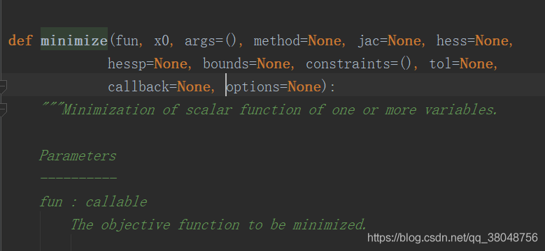
//Here's the declaration. I think it's a good idea to check the function's description.
def minimize(fun, x0, args=(), method=None, jac=None, hess=None,
             hessp=None, bounds=None, constraints=(), tol=None,
             callback=None, options=None):
fun : this parameter is the costFunction that you want to minimize the loss of. Pass the name of costFunction to fun
.
The objective function to be minimized.
fun(x, *args) -> float
where x is an 1-D array with shape (n,) and args
is a tuple of the fixed parameters needed to completely
specify the function.
This means that when the loss function is defined, ** must be the first argument and its shape must be (n,)**, a one-dimensional array. Other parameters used in the calculation of the loss function are passed into the args parameters (other parameters specifically refer to X, Y, lambda, etc.) in the form of tuples, and finally return the loss value, which can be in the form of an array or a real number.
The parameter x0 is initialized to theta, whose shape must be shape(n,), which is a one-dimensional array.
method : this parameter represents the way to be adopted, default is one of BFGS, l-bfgs-b , SLSQP, optional TNC
jac : this parameter is a function to calculate the gradient. Similar to the fun parameter, the first parameter must be theta and its shape must be (n,), which is a one-dimensional array. The gradient returned at the end must also be a one-dimensional array.
options : used to control the maximum number of iterations and set in the form of a dictionary, for example: options={‘ maxiter ‘:400}
The parameters used are mainly these, and the application examples are as follows (where Ng’s machine learning EX2 is used) :
def costFunction(theta,X,Y,lmd):
    theta = theta.reshape((len(theta), 1))
    Y=Y.reshape(len(Y),1)
    m=X.shape[0]
    J=0
    first=-(Y.T)@np.log(sigmoid(X@theta))
    second=(1-Y.T)@np.log(1-sigmoid(X@theta))
    theta2=theta[1:,:]
    assert (theta2.shape==(theta.size-1,1))
    J=(first-second)/m+lmd/(2*m)*(theta2.T@theta2)
    return J
def gradient(theta,X,Y,lmd):
    theta = theta.reshape((len(theta), 1))
    Y = Y.reshape(len(Y), 1)
    reg = (lmd/len(X)) * theta
    reg[0] = 0
    grad=(X.T @ (sigmoid(X @ theta) - Y))/len(X)
    return (grad+reg).ravel()

result=op.minimize(fun=costFunction,x0=theta.reshape(28,),args=(X,Y,1),method='TNC',jac=gradient,options={'maxiter':400})
print(result)
final_theta = result.x
Output:
fun: array([[0.52900273]])
     jac: array([-2.15010332e-06,  6.79564299e-07, -3.48680372e-07,  8.76012223e-07,
       -4.07509002e-08, -9.33423708e-07, -5.14520466e-07,  1.71377727e-08,
        1.55330746e-08, -9.72472529e-07,  6.96683054e-08,  3.55303286e-08,
       -2.79411735e-07,  1.79649627e-07,  2.33480997e-07,  1.47186558e-07,
       -2.11705227e-07,  6.16713286e-07, -9.29181534e-08, -5.27541662e-08,
       -1.48146987e-06,  2.31241473e-07,  1.80347588e-07, -1.31898660e-07,
       -7.16759904e-08, -4.12328300e-07,  1.65360544e-08, -7.34643861e-07])
 message: 'Converged (|f_n-f_(n-1)| ~= 0)'
    nfev: 32
     nit: 7
  status: 1
 success: True
       x: array([ 1.27271027,  0.62529965,  1.18111686, -2.019874  , -0.91743189,
       -1.4316693 ,  0.12393227, -0.36553118, -0.35725403, -0.17516292,
       -1.45817009, -0.05098418, -0.61558553, -0.27469166, -1.19271298,
       -0.2421784 , -0.20603297, -0.04466178, -0.27778952, -0.29539513,
       -0.45645982, -1.04319155,  0.02779373, -0.29244871,  0.0155576 ,
       -0.32742406, -0.1438915 , -0.92467487])
1. The X0 parameter is the initialized theta, which must be a one-dimensional array, and the gradient return value must be a one-dimensional array, i.e., the gradient is stored as a one-dimensional array.
2. An array using the attention to the shape, to learn how to reasonable use reshape make sure it is operating. 3. For one-dimensional array a=[0,1,2,3], a[0]. Shape =(), a[0]. Size =1.
3. Minimize the solution of constraint functions
Fun: To find the minimum target function
X0: The initial guess for the variable. If there are multiple variables, you need to give each one an initial guess. Minimize the occurrence of local optimality, so it is necessary to find a means of dealing with it.
Args: constant values, as will be explained in the following examples. There are no Numbers in FUN, but they are expressed in the form of variables. For constant terms, we need to give a value here
Method: There are many ways to find an extreme value. The default is generally used. Each method I understand is to calculate the error, the way of back propagation is different, this area has a lot of theoretical research space
Constraints: Constraints that constrain the part of FUN that is the parameter
1.Calculate the minimum value of 1/x+x
# coding=utf-8
from scipy.optimize import minimize
import numpy as np
#demo 1
#Calculate the minimum value of 1/x+x
def fun(args):
a=args
v=lambda x:a/x[0] +x[0]
return v
if __name__ == "__main__":
args = (1) #a
x0 = np.asarray((2)) # Initial guesses
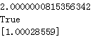
res = minimize(fun(args), x0, method='SLSQP')
print(res.fun)
print(res.success)
print(res.x)
Results: the function of the minimum value for more than 2 points
the block reference link: https://blog.csdn.net/ljyljyok/article/details/100552618
4. It is a minimize function
Scipy api:https://docs.scipy.org/doc/scipy-0.18.1/reference/index.html
"""
Unified interfaces to minimization algorithms.
Functions
---------
- minimize : minimization of a function of several variables.
- minimize_scalar : minimization of a function of one variable.
"""
from __future__ import division, print_function, absolute_import
__all__ = ['minimize', 'minimize_scalar']
from warnings import warn
import numpy as np
from scipy._lib.six import callable
from scipy.sparse.linalg import LinearOperator
# unconstrained minimization
from .optimize import (_minimize_neldermead, _minimize_powell, _minimize_cg,
_minimize_bfgs, _minimize_newtoncg,
_minimize_scalar_brent, _minimize_scalar_bounded,
_minimize_scalar_golden, MemoizeJac)
from ._trustregion_dogleg import _minimize_dogleg
from ._trustregion_ncg import _minimize_trust_ncg
from ._trustregion_krylov import _minimize_trust_krylov
from ._trustregion_exact import _minimize_trustregion_exact
from ._trustregion_constr import _minimize_trustregion_constr
from ._constraints import Bounds, new_bounds_to_old, old_bound_to_new
# constrained minimization
from .lbfgsb import _minimize_lbfgsb
from .tnc import _minimize_tnc
from .cobyla import _minimize_cobyla
from .slsqp import _minimize_slsqp
def minimize(fun, x0, args=(), method=None, jac=None, hess=None,
hessp=None, bounds=None, constraints=(), tol=None,
callback=None, options=None):
"""Minimization of scalar function of one or more variables.
Parameters
----------
fun : callable
The objective function to be minimized.
``fun(x, *args) -> float``
where x is an 1-D array with shape (n,) and `args`
is a tuple of the fixed parameters needed to completely
specify the function.
x0 : ndarray, shape (n,)
Initial guess. Array of real elements of size (n,),
where 'n' is the number of independent variables.
args : tuple, optional
Extra arguments passed to the objective function and its
derivatives (`fun`, `jac` and `hess` functions).
method : str or callable, optional
Type of solver. Should be one of
- 'Nelder-Mead' :ref:`(see here) <optimize.minimize-neldermead>`
- 'Powell' :ref:`(see here) <optimize.minimize-powell>`
- 'CG' :ref:`(see here) <optimize.minimize-cg>`
- 'BFGS' :ref:`(see here) <optimize.minimize-bfgs>`
- 'Newton-CG' :ref:`(see here) <optimize.minimize-newtoncg>`
- 'L-BFGS-B' :ref:`(see here) <optimize.minimize-lbfgsb>`
- 'TNC' :ref:`(see here) <optimize.minimize-tnc>`
- 'COBYLA' :ref:`(see here) <optimize.minimize-cobyla>`
- 'SLSQP' :ref:`(see here) <optimize.minimize-slsqp>`
- 'trust-constr':ref:`(see here) <optimize.minimize-trustconstr>`
- 'dogleg' :ref:`(see here) <optimize.minimize-dogleg>`
- 'trust-ncg' :ref:`(see here) <optimize.minimize-trustncg>`
- 'trust-exact' :ref:`(see here) <optimize.minimize-trustexact>`
- 'trust-krylov' :ref:`(see here) <optimize.minimize-trustkrylov>`
- custom - a callable object (added in version 0.14.0),
see below for description.
If not given, chosen to be one of ``BFGS``, ``L-BFGS-B``, ``SLSQP``,
depending if the problem has constraints or bounds.
jac : {callable, '2-point', '3-point', 'cs', bool}, optional
Method for computing the gradient vector. Only for CG, BFGS,
Newton-CG, L-BFGS-B, TNC, SLSQP, dogleg, trust-ncg, trust-krylov,
trust-exact and trust-constr. If it is a callable, it should be a
function that returns the gradient vector:
``jac(x, *args) -> array_like, shape (n,)``
where x is an array with shape (n,) and `args` is a tuple with
the fixed parameters. Alternatively, the keywords
{'2-point', '3-point', 'cs'} select a finite
difference scheme for numerical estimation of the gradient. Options
'3-point' and 'cs' are available only to 'trust-constr'.
If `jac` is a Boolean and is True, `fun` is assumed to return the
gradient along with the objective function. If False, the gradient
will be estimated using '2-point' finite difference estimation.
hess : {callable, '2-point', '3-point', 'cs', HessianUpdateStrategy}, optional
Method for computing the Hessian matrix. Only for Newton-CG, dogleg,
trust-ncg, trust-krylov, trust-exact and trust-constr. If it is
callable, it should return the Hessian matrix:
``hess(x, *args) -> {LinearOperator, spmatrix, array}, (n, n)``
where x is a (n,) ndarray and `args` is a tuple with the fixed
parameters. LinearOperator and sparse matrix returns are
allowed only for 'trust-constr' method. Alternatively, the keywords
{'2-point', '3-point', 'cs'} select a finite difference scheme
for numerical estimation. Or, objects implementing
`HessianUpdateStrategy` interface can be used to approximate
the Hessian. Available quasi-Newton methods implementing
this interface are:
- `BFGS`;
- `SR1`.
Whenever the gradient is estimated via finite-differences,
the Hessian cannot be estimated with options
{'2-point', '3-point', 'cs'} and needs to be
estimated using one of the quasi-Newton strategies.
Finite-difference options {'2-point', '3-point', 'cs'} and
`HessianUpdateStrategy` are available only for 'trust-constr' method.
hessp : callable, optional
Hessian of objective function times an arbitrary vector p. Only for
Newton-CG, trust-ncg, trust-krylov, trust-constr.
Only one of `hessp` or `hess` needs to be given. If `hess` is
provided, then `hessp` will be ignored. `hessp` must compute the
Hessian times an arbitrary vector:
``hessp(x, p, *args) -> ndarray shape (n,)``
where x is a (n,) ndarray, p is an arbitrary vector with
dimension (n,) and `args` is a tuple with the fixed
parameters.
bounds : sequence or `Bounds`, optional
Bounds on variables for L-BFGS-B, TNC, SLSQP and
trust-constr methods. There are two ways to specify the bounds:
1. Instance of `Bounds` class.
2. Sequence of ``(min, max)`` pairs for each element in `x`. None
is used to specify no bound.
constraints : {Constraint, dict} or List of {Constraint, dict}, optional
Constraints definition (only for COBYLA, SLSQP and trust-constr).
Constraints for 'trust-constr' are defined as a single object or a
list of objects specifying constraints to the optimization problem.
Available constraints are:
- `LinearConstraint`
- `NonlinearConstraint`
Constraints for COBYLA, SLSQP are defined as a list of dictionaries.
Each dictionary with fields:
type : str
Constraint type: 'eq' for equality, 'ineq' for inequality.
fun : callable
The function defining the constraint.
jac : callable, optional
The Jacobian of `fun` (only for SLSQP).
args : sequence, optional
Extra arguments to be passed to the function and Jacobian.
Equality constraint means that the constraint function result is to
be zero whereas inequality means that it is to be non-negative.
Note that COBYLA only supports inequality constraints.
tol : float, optional
Tolerance for termination. For detailed control, use solver-specific
options.
options : dict, optional
A dictionary of solver options. All methods accept the following
generic options:
maxiter : int
Maximum number of iterations to perform.
disp : bool
Set to True to print convergence messages.
For method-specific options, see :func:`show_options()`.
callback : callable, optional
Called after each iteration. For 'trust-constr' it is a callable with
the signature:
``callback(xk, OptimizeResult state) -> bool``
where ``xk`` is the current parameter vector. and ``state``
is an `OptimizeResult` object, with the same fields
as the ones from the return. If callback returns True
the algorithm execution is terminated.
For all the other methods, the signature is:
``callback(xk)``
where ``xk`` is the current parameter vector.
Returns
-------
res : OptimizeResult
The optimization result represented as a ``OptimizeResult`` object.
Important attributes are: ``x`` the solution array, ``success`` a
Boolean flag indicating if the optimizer exited successfully and
``message`` which describes the cause of the termination. See
`OptimizeResult` for a description of other attributes.
See also
--------
minimize_scalar : Interface to minimization algorithms for scalar
univariate functions
show_options : Additional options accepted by the solvers
Notes
-----
This section describes the available solvers that can be selected by the
'method' parameter. The default method is *BFGS*.
**Unconstrained minimization**
Method :ref:`Nelder-Mead <optimize.minimize-neldermead>` uses the
Simplex algorithm [1]_, [2]_. This algorithm is robust in many
applications. However, if numerical computation of derivative can be
trusted, other algorithms using the first and/or second derivatives
information might be preferred for their better performance in
general.
Method :ref:`Powell <optimize.minimize-powell>` is a modification
of Powell's method [3]_, [4]_ which is a conjugate direction
method. It performs sequential one-dimensional minimizations along
each vector of the directions set (`direc` field in `options` and
`info`), which is updated at each iteration of the main
minimization loop. The function need not be differentiable, and no
derivatives are taken.
Method :ref:`CG <optimize.minimize-cg>` uses a nonlinear conjugate
gradient algorithm by Polak and Ribiere, a variant of the
Fletcher-Reeves method described in [5]_ pp. 120-122. Only the
first derivatives are used.
Method :ref:`BFGS <optimize.minimize-bfgs>` uses the quasi-Newton
method of Broyden, Fletcher, Goldfarb, and Shanno (BFGS) [5]_
pp. 136. It uses the first derivatives only. BFGS has proven good
performance even for non-smooth optimizations. This method also
returns an approximation of the Hessian inverse, stored as
`hess_inv` in the OptimizeResult object.
Method :ref:`Newton-CG <optimize.minimize-newtoncg>` uses a
Newton-CG algorithm [5]_ pp. 168 (also known as the truncated
Newton method). It uses a CG method to the compute the search
direction. See also *TNC* method for a box-constrained
minimization with a similar algorithm. Suitable for large-scale
problems.
Method :ref:`dogleg <optimize.minimize-dogleg>` uses the dog-leg
trust-region algorithm [5]_ for unconstrained minimization. This
algorithm requires the gradient and Hessian; furthermore the
Hessian is required to be positive definite.
Method :ref:`trust-ncg <optimize.minimize-trustncg>` uses the
Newton conjugate gradient trust-region algorithm [5]_ for
unconstrained minimization. This algorithm requires the gradient
and either the Hessian or a function that computes the product of
the Hessian with a given vector. Suitable for large-scale problems.
Method :ref:`trust-krylov <optimize.minimize-trustkrylov>` uses
the Newton GLTR trust-region algorithm [14]_, [15]_ for unconstrained
minimization. This algorithm requires the gradient
and either the Hessian or a function that computes the product of
the Hessian with a given vector. Suitable for large-scale problems.
On indefinite problems it requires usually less iterations than the
`trust-ncg` method and is recommended for medium and large-scale problems.
Method :ref:`trust-exact <optimize.minimize-trustexact>`
is a trust-region method for unconstrained minimization in which
quadratic subproblems are solved almost exactly [13]_. This
algorithm requires the gradient and the Hessian (which is
*not* required to be positive definite). It is, in many
situations, the Newton method to converge in fewer iteraction
and the most recommended for small and medium-size problems.
**Bound-Constrained minimization**
Method :ref:`L-BFGS-B <optimize.minimize-lbfgsb>` uses the L-BFGS-B
algorithm [6]_, [7]_ for bound constrained minimization.
Method :ref:`TNC <optimize.minimize-tnc>` uses a truncated Newton
algorithm [5]_, [8]_ to minimize a function with variables subject
to bounds. This algorithm uses gradient information; it is also
called Newton Conjugate-Gradient. It differs from the *Newton-CG*
method described above as it wraps a C implementation and allows
each variable to be given upper and lower bounds.
**Constrained Minimization**
Method :ref:`COBYLA <optimize.minimize-cobyla>` uses the
Constrained Optimization BY Linear Approximation (COBYLA) method
[9]_, [10]_, [11]_. The algorithm is based on linear
approximations to the objective function and each constraint. The
method wraps a FORTRAN implementation of the algorithm. The
constraints functions 'fun' may return either a single number
or an array or list of numbers.
Method :ref:`SLSQP <optimize.minimize-slsqp>` uses Sequential
Least SQuares Programming to minimize a function of several
variables with any combination of bounds, equality and inequality
constraints. The method wraps the SLSQP Optimization subroutine
originally implemented by Dieter Kraft [12]_. Note that the
wrapper handles infinite values in bounds by converting them into
large floating values.
Method :ref:`trust-constr <optimize.minimize-trustconstr>` is a
trust-region algorithm for constrained optimization. It swiches
between two implementations depending on the problem definition.
It is the most versatile constrained minimization algorithm
implemented in SciPy and the most appropriate for large-scale problems.
For equality constrained problems it is an implementation of Byrd-Omojokun
Trust-Region SQP method described in [17]_ and in [5]_, p. 549. When
inequality constraints are imposed as well, it swiches to the trust-region
interior point method described in [16]_. This interior point algorithm,
in turn, solves inequality constraints by introducing slack variables
and solving a sequence of equality-constrained barrier problems
for progressively smaller values of the barrier parameter.
The previously described equality constrained SQP method is
used to solve the subproblems with increasing levels of accuracy
as the iterate gets closer to a solution.
**Finite-Difference Options**
For Method :ref:`trust-constr <optimize.minimize-trustconstr>`
the gradient and the Hessian may be approximated using
three finite-difference schemes: {'2-point', '3-point', 'cs'}.
The scheme 'cs' is, potentially, the most accurate but it
requires the function to correctly handles complex inputs and to
be differentiable in the complex plane. The scheme '3-point' is more
accurate than '2-point' but requires twice as much operations.
**Custom minimizers**
It may be useful to pass a custom minimization method, for example
when using a frontend to this method such as `scipy.optimize.basinhopping`
or a different library. You can simply pass a callable as the ``method``
parameter.
The callable is called as ``method(fun, x0, args, **kwargs, **options)``
where ``kwargs`` corresponds to any other parameters passed to `minimize`
(such as `callback`, `hess`, etc.), except the `options` dict, which has
its contents also passed as `method` parameters pair by pair. Also, if
`jac` has been passed as a bool type, `jac` and `fun` are mangled so that
`fun` returns just the function values and `jac` is converted to a function
returning the Jacobian. The method shall return an ``OptimizeResult``
object.
The provided `method` callable must be able to accept (and possibly ignore)
arbitrary parameters; the set of parameters accepted by `minimize` may
expand in future versions and then these parameters will be passed to
the method. You can find an example in the scipy.optimize tutorial.
.. versionadded:: 0.11.0
References
----------
.. [1] Nelder, J A, and R Mead. 1965. A Simplex Method for Function
Minimization. The Computer Journal 7: 308-13.
.. [2] Wright M H. 1996. Direct search methods: Once scorned, now
respectable, in Numerical Analysis 1995: Proceedings of the 1995
Dundee Biennial Conference in Numerical Analysis (Eds. D F
Griffiths and G A Watson). Addison Wesley Longman, Harlow, UK.
191-208.
.. [3] Powell, M J D. 1964. An efficient method for finding the minimum of
a function of several variables without calculating derivatives. The
Computer Journal 7: 155-162.
.. [4] Press W, S A Teukolsky, W T Vetterling and B P Flannery.
Numerical Recipes (any edition), Cambridge University Press.
.. [5] Nocedal, J, and S J Wright. 2006. Numerical Optimization.
Springer New York.
.. [6] Byrd, R H and P Lu and J. Nocedal. 1995. A Limited Memory
Algorithm for Bound Constrained Optimization. SIAM Journal on
Scientific and Statistical Computing 16 (5): 1190-1208.
.. [7] Zhu, C and R H Byrd and J Nocedal. 1997. L-BFGS-B: Algorithm
778: L-BFGS-B, FORTRAN routines for large scale bound constrained
optimization. ACM Transactions on Mathematical Software 23 (4):
550-560.
.. [8] Nash, S G. Newton-Type Minimization Via the Lanczos Method.
1984. SIAM Journal of Numerical Analysis 21: 770-778.
.. [9] Powell, M J D. A direct search optimization method that models
the objective and constraint functions by linear interpolation.
1994. Advances in Optimization and Numerical Analysis, eds. S. Gomez
and J-P Hennart, Kluwer Academic (Dordrecht), 51-67.
.. [10] Powell M J D. Direct search algorithms for optimization
calculations. 1998. Acta Numerica 7: 287-336.
.. [11] Powell M J D. A view of algorithms for optimization without
derivatives. 2007.Cambridge University Technical Report DAMTP
2007/NA03
.. [12] Kraft, D. A software package for sequential quadratic
programming. 1988. Tech. Rep. DFVLR-FB 88-28, DLR German Aerospace
Center -- Institute for Flight Mechanics, Koln, Germany.
.. [13] Conn, A. R., Gould, N. I., and Toint, P. L.
Trust region methods. 2000. Siam. pp. 169-200.
.. [14] F. Lenders, C. Kirches, A. Potschka: "trlib: A vector-free
implementation of the GLTR method for iterative solution of
the trust region problem", https://arxiv.org/abs/1611.04718
.. [15] N. Gould, S. Lucidi, M. Roma, P. Toint: "Solving the
Trust-Region Subproblem using the Lanczos Method",
SIAM J. Optim., 9(2), 504--525, (1999).
.. [16] Byrd, Richard H., Mary E. Hribar, and Jorge Nocedal. 1999.
An interior point algorithm for large-scale nonlinear programming.
SIAM Journal on Optimization 9.4: 877-900.
.. [17] Lalee, Marucha, Jorge Nocedal, and Todd Plantega. 1998. On the
implementation of an algorithm for large-scale equality constrained
optimization. SIAM Journal on Optimization 8.3: 682-706.
Examples
--------
Let us consider the problem of minimizing the Rosenbrock function. This
function (and its respective derivatives) is implemented in `rosen`
(resp. `rosen_der`, `rosen_hess`) in the `scipy.optimize`.
>>> from scipy.optimize import minimize, rosen, rosen_der
A simple application of the *Nelder-Mead* method is:
>>> x0 = [1.3, 0.7, 0.8, 1.9, 1.2]
>>> res = minimize(rosen, x0, method='Nelder-Mead', tol=1e-6)
>>> res.x
array([ 1., 1., 1., 1., 1.])
Now using the *BFGS* algorithm, using the first derivative and a few
options:
>>> res = minimize(rosen, x0, method='BFGS', jac=rosen_der,
... options={'gtol': 1e-6, 'disp': True})
Optimization terminated successfully.
Current function value: 0.000000
Iterations: 26
Function evaluations: 31
Gradient evaluations: 31
>>> res.x
array([ 1., 1., 1., 1., 1.])
>>> print(res.message)
Optimization terminated successfully.
>>> res.hess_inv
array([[ 0.00749589, 0.01255155, 0.02396251, 0.04750988, 0.09495377], # may vary
[ 0.01255155, 0.02510441, 0.04794055, 0.09502834, 0.18996269],
[ 0.02396251, 0.04794055, 0.09631614, 0.19092151, 0.38165151],
[ 0.04750988, 0.09502834, 0.19092151, 0.38341252, 0.7664427 ],
[ 0.09495377, 0.18996269, 0.38165151, 0.7664427, 1.53713523]])
Next, consider a minimization problem with several constraints (namely
Example 16.4 from [5]_). The objective function is:
>>> fun = lambda x: (x[0] - 1)**2 + (x[1] - 2.5)**2
There are three constraints defined as:
>>> cons = ({'type': 'ineq', 'fun': lambda x: x[0] - 2 * x[1] + 2},
... {'type': 'ineq', 'fun': lambda x: -x[0] - 2 * x[1] + 6},
... {'type': 'ineq', 'fun': lambda x: -x[0] + 2 * x[1] + 2})
And variables must be positive, hence the following bounds:
>>> bnds = ((0, None), (0, None))
The optimization problem is solved using the SLSQP method as:
>>> res = minimize(fun, (2, 0), method='SLSQP', bounds=bnds,
... constraints=cons)
It should converge to the theoretical solution (1.4 ,1.7).
"""
x0 = np.asarray(x0)
if x0.dtype.kind in np.typecodes["AllInteger"]:
x0 = np.asarray(x0, dtype=float)
if not isinstance(args, tuple):
args = (args,)
if method is None:
# Select automatically
if constraints:
method = 'SLSQP'
elif bounds is not None:
method = 'L-BFGS-B'
else:
method = 'BFGS'
if callable(method):
meth = "_custom"
else:
meth = method.lower()
if options is None:
options = {}
# check if optional parameters are supported by the selected method
# - jac
if meth in ('nelder-mead', 'powell', 'cobyla') and bool(jac):
warn('Method %s does not use gradient information (jac).' % method,
RuntimeWarning)
# - hess
if meth not in ('newton-cg', 'dogleg', 'trust-ncg', 'trust-constr',
'trust-krylov', 'trust-exact', '_custom') and hess is not None:
warn('Method %s does not use Hessian information (hess).' % method,
RuntimeWarning)
# - hessp
if meth not in ('newton-cg', 'dogleg', 'trust-ncg', 'trust-constr',
'trust-krylov', '_custom') \
and hessp is not None:
warn('Method %s does not use Hessian-vector product '
'information (hessp).' % method, RuntimeWarning)
# - constraints or bounds
if (meth in ('nelder-mead', 'powell', 'cg', 'bfgs', 'newton-cg', 'dogleg',
'trust-ncg') and (bounds is not None or np.any(constraints))):
warn('Method %s cannot handle constraints nor bounds.' % method,
RuntimeWarning)
if meth in ('l-bfgs-b', 'tnc') and np.any(constraints):
warn('Method %s cannot handle constraints.' % method,
RuntimeWarning)
if meth == 'cobyla' and bounds is not None:
warn('Method %s cannot handle bounds.' % method,
RuntimeWarning)
# - callback
if (meth in ('cobyla',) and callback is not None):
warn('Method %s does not support callback.' % method, RuntimeWarning)
# - return_all
if (meth in ('l-bfgs-b', 'tnc', 'cobyla', 'slsqp') and
options.get('return_all', False)):
warn('Method %s does not support the return_all option.' % method,
RuntimeWarning)
# check gradient vector
if meth == 'trust-constr':
if type(jac) is bool:
if jac:
fun = MemoizeJac(fun)
jac = fun.derivative
else:
jac = '2-point'
elif not callable(jac) and jac not in ('2-point', '3-point', 'cs'):
raise ValueError("Unsupported jac definition.")
else:
if jac in ('2-point', '3-point', 'cs'):
if jac in ('3-point', 'cs'):
warn("Only 'trust-constr' method accept %s "
"options for 'jac'. Using '2-point' instead." % jac)
jac = None
elif not callable(jac):
if bool(jac):
fun = MemoizeJac(fun)
jac = fun.derivative
else:
jac = None
# set default tolerances
if tol is not None:
options = dict(options)
if meth == 'nelder-mead':
options.setdefault('xatol', tol)
options.setdefault('fatol', tol)
if meth in ('newton-cg', 'powell', 'tnc'):
options.setdefault('xtol', tol)
if meth in ('powell', 'l-bfgs-b', 'tnc', 'slsqp'):
options.setdefault('ftol', tol)
if meth in ('bfgs', 'cg', 'l-bfgs-b', 'tnc', 'dogleg',
'trust-ncg', 'trust-exact', 'trust-krylov'):
options.setdefault('gtol', tol)
if meth in ('cobyla', '_custom'):
options.setdefault('tol', tol)
if meth == 'trust-constr':
options.setdefault('xtol', tol)
options.setdefault('gtol', tol)
options.setdefault('barrier_tol', tol)
if bounds is not None:
if meth == 'trust-constr':
if not isinstance(bounds, Bounds):
lb, ub = old_bound_to_new(bounds)
bounds = Bounds(lb, ub)
elif meth in ('l-bfgs-b', 'tnc', 'slsqp'):
if isinstance(bounds, Bounds):
bounds = new_bounds_to_old(bounds.lb, bounds.ub, x0.shape[0])
if meth == '_custom':
return method(fun, x0, args=args, jac=jac, hess=hess, hessp=hessp,
bounds=bounds, constraints=constraints,
callback=callback, **options)
elif meth == 'nelder-mead':
return _minimize_neldermead(fun, x0, args, callback, **options)
elif meth == 'powell':
return _minimize_powell(fun, x0, args, callback, **options)
elif meth == 'cg':
return _minimize_cg(fun, x0, args, jac, callback, **options)
elif meth == 'bfgs':
return _minimize_bfgs(fun, x0, args, jac, callback, **options)
elif meth == 'newton-cg':
return _minimize_newtoncg(fun, x0, args, jac, hess, hessp, callback,
**options)
elif meth == 'l-bfgs-b':
return _minimize_lbfgsb(fun, x0, args, jac, bounds,
callback=callback, **options)
elif meth == 'tnc':
return _minimize_tnc(fun, x0, args, jac, bounds, callback=callback,
**options)
elif meth == 'cobyla':
return _minimize_cobyla(fun, x0, args, constraints, **options)
elif meth == 'slsqp':
return _minimize_slsqp(fun, x0, args, jac, bounds,
constraints, callback=callback, **options)
elif meth == 'trust-constr':
return _minimize_trustregion_constr(fun, x0, args, jac, hess, hessp,
bounds, constraints,
callback=callback, **options)
elif meth == 'dogleg':
return _minimize_dogleg(fun, x0, args, jac, hess,
callback=callback, **options)
elif meth == 'trust-ncg':
return _minimize_trust_ncg(fun, x0, args, jac, hess, hessp,
callback=callback, **options)
elif meth == 'trust-krylov':
return _minimize_trust_krylov(fun, x0, args, jac, hess, hessp,
callback=callback, **options)
elif meth == 'trust-exact':
return _minimize_trustregion_exact(fun, x0, args, jac, hess,
callback=callback, **options)
else:
raise ValueError('Unknown solver %s' % method)
def minimize_scalar(fun, bracket=None, bounds=None, args=(),
method='brent', tol=None, options=None):
"""Minimization of scalar function of one variable.
Parameters
----------
fun : callable
Objective function.
Scalar function, must return a scalar.
bracket : sequence, optional
For methods 'brent' and 'golden', `bracket` defines the bracketing
interval and can either have three items ``(a, b, c)`` so that
``a < b < c`` and ``fun(b) < fun(a), fun(c)`` or two items ``a`` and
``c`` which are assumed to be a starting interval for a downhill
bracket search (see `bracket`); it doesn't always mean that the
obtained solution will satisfy ``a <= x <= c``.
bounds : sequence, optional
For method 'bounded', `bounds` is mandatory and must have two items
corresponding to the optimization bounds.
args : tuple, optional
Extra arguments passed to the objective function.
method : str or callable, optional
Type of solver. Should be one of:
- 'Brent' :ref:`(see here) <optimize.minimize_scalar-brent>`
- 'Bounded' :ref:`(see here) <optimize.minimize_scalar-bounded>`
- 'Golden' :ref:`(see here) <optimize.minimize_scalar-golden>`
- custom - a callable object (added in version 0.14.0), see below
tol : float, optional
Tolerance for termination. For detailed control, use solver-specific
options.
options : dict, optional
A dictionary of solver options.
maxiter : int
Maximum number of iterations to perform.
disp : bool
Set to True to print convergence messages.
See :func:`show_options()` for solver-specific options.
Returns
-------
res : OptimizeResult
The optimization result represented as a ``OptimizeResult`` object.
Important attributes are: ``x`` the solution array, ``success`` a
Boolean flag indicating if the optimizer exited successfully and
``message`` which describes the cause of the termination. See
`OptimizeResult` for a description of other attributes.
See also
--------
minimize : Interface to minimization algorithms for scalar multivariate
functions
show_options : Additional options accepted by the solvers
Notes
-----
This section describes the available solvers that can be selected by the
'method' parameter. The default method is *Brent*.
Method :ref:`Brent <optimize.minimize_scalar-brent>` uses Brent's
algorithm to find a local minimum. The algorithm uses inverse
parabolic interpolation when possible to speed up convergence of
the golden section method.
Method :ref:`Golden <optimize.minimize_scalar-golden>` uses the
golden section search technique. It uses analog of the bisection
method to decrease the bracketed interval. It is usually
preferable to use the *Brent* method.
Method :ref:`Bounded <optimize.minimize_scalar-bounded>` can
perform bounded minimization. It uses the Brent method to find a
local minimum in the interval x1 < xopt < x2.
**Custom minimizers**
It may be useful to pass a custom minimization method, for example
when using some library frontend to minimize_scalar. You can simply
pass a callable as the ``method`` parameter.
The callable is called as ``method(fun, args, **kwargs, **options)``
where ``kwargs`` corresponds to any other parameters passed to `minimize`
(such as `bracket`, `tol`, etc.), except the `options` dict, which has
its contents also passed as `method` parameters pair by pair. The method
shall return an ``OptimizeResult`` object.
The provided `method` callable must be able to accept (and possibly ignore)
arbitrary parameters; the set of parameters accepted by `minimize` may
expand in future versions and then these parameters will be passed to
the method. You can find an example in the scipy.optimize tutorial.
.. versionadded:: 0.11.0
Examples
--------
Consider the problem of minimizing the following function.
>>> def f(x):
... return (x - 2) * x * (x + 2)**2
Using the *Brent* method, we find the local minimum as:
>>> from scipy.optimize import minimize_scalar
>>> res = minimize_scalar(f)
>>> res.x
1.28077640403
Using the *Bounded* method, we find a local minimum with specified
bounds as:
>>> res = minimize_scalar(f, bounds=(-3, -1), method='bounded')
>>> res.x
-2.0000002026
"""
if not isinstance(args, tuple):
args = (args,)
if callable(method):
meth = "_custom"
else:
meth = method.lower()
if options is None:
options = {}
if tol is not None:
options = dict(options)
if meth == 'bounded' and 'xatol' not in options:
warn("Method 'bounded' does not support relative tolerance in x; "
"defaulting to absolute tolerance.", RuntimeWarning)
options['xatol'] = tol
elif meth == '_custom':
options.setdefault('tol', tol)
else:
options.setdefault('xtol', tol)
if meth == '_custom':
return method(fun, args=args, bracket=bracket, bounds=bounds, **options)
elif meth == 'brent':
return _minimize_scalar_brent(fun, bracket, args, **options)
elif meth == 'bounded':
if bounds is None:
raise ValueError('The `bounds` parameter is mandatory for '
'method `bounded`.')
# replace boolean "disp" option, if specified, by an integer value, as
# expected by _minimize_scalar_bounded()
disp = options.get('disp')
if isinstance(disp, bool):
options['disp'] = 2 * int(disp)
return _minimize_scalar_bounded(fun, bounds, args, **options)
elif meth == 'golden':
return _minimize_scalar_golden(fun, bracket, args, **options)
else:
raise ValueError('Unknown solver %s' % method)
Read More:
- Detailed explanation of OpenCV approxpolydp() function
- [Solved] RuntimeError: function ALSQPlusBackward returned a gradient different than None at position 3, but t
- To silence this warning, use `float` by itself. Doing this will not modify any behavior and is safe.
- [Python] How to Sort a Group of Tuples Using the Sorted() Function
- Opencv Python realizes the paint filling function in PS, one click filling color and the possible reasons for opencv’s frequent errors
- error: (-5:Bad argument) in function ‘seamlessClone‘ and error: (-215:Assertion failed) 0 <= roi.x && 0 [How to Solve]
- Python: Torch.nn.functional.normalize() Function
- torch.nn.functional.normalize() Function Interpretation
- Python+OpenCV: How to Use Background Subtraction Methods
- [Solved] Request.url is not modifiable, use Request.replace() instead
- [Pytorch Error Solution] Pytorch distributed RuntimeError: Address already in use
- [Solved] Pdfplumber Read PDF Sheet Error: AttributeError: function/symbol ‘ARC4_stream_init‘ not found in library
- Plt.acorr() Function Error: ValueError: object too deep for desired array
- [Solved] python opencv Error: findContours() Can only use the Grayscale
- [Solved] error: (-215:Assertion failed) !_src.empty() in function ‘cv::cvtColor‘
- python Use timeit Error: stmt is neither a string nor callable
- Python: How to Use os.path.join()
- RuntimeError: Address already in use [How to Solve]
- [Solved] cv2.error: OpenCV(4.5.3) :-1: error: (-5:Bad argument) in function ‘circle‘
- [Solved] error: (-2:Unspecified error) The function is not implemented. Rebuild the library with Windows