Tag Archives: R

Error in value[[3L]](cond) : Package ‘rhdf5‘ version 2.36.0 cannot be unloaded:

library(rhdf5)
Error in value[[3L]](cond) : Package 'rhdf5' version 2.36.0 cannot be unloaded:Error in unloadNamespace(package) : namespace 'rhdf5' is imported by 'HDF5Array', 'MOFA2' so cannot be unloaded

This is caused by importing packages from two places

Solution:

unloadNamespace('MOFA2')
unloadNamespace('HDF5Array')
library(rhdf5)

success

[Solved] R Error: Python module tensorflow.keras was not found.

Scenario:

rstudio reported error R: Python module tensorflow.keras was not found.
at first, I suspected that I could not accurately locate the keras package of R, because I was using Anaconda to do other things, but later I saw other error reports and felt that they were not so complex… Later, I found that they were just simple and not installed properly… In short, the solution is as follows


Solution:

terminal input:

install.packages(tensorflow)
install_tensorflow()
library(tensorflow)
#Keras The R interface uses the TensorFlow backend engine.
# To install the core Keras library and TensorFlow backend, use the install_keras() function
install_keras()
library(keras)
# Run them all and then tune the package, if you have already done so, restart RStudio
-------------------------------------------
#Other solutions to this problem are as follows:
library(tensorflow)
library(keras)
use_condaenv("r-tensorflow")

RCurl error-fatal error: curl/curl.h: No such file or directory

# R version 4.1.1 (2021-08-10)
install.packages("E:/R/R-4.1.1/library/RCurl_1.98-1.4.tar.gz", repos = NULL, type = "source")

The operation process is as follows:

* installing *source* package 'RCurl' ...
** package 'RCurl' successfully unpacked and MD5 sums checked
** using staged installation
** libs

*** arch - i386
"E:/R/rtools40/mingw32/bin/"gcc  -I"E:/R/R-41~1.1/include" -DNDEBUG -I/include -DHAVE_LIBIDN_FIELD=1 -DHAVE_CURLOPT_URL=1 -DHAVE_CURLINFO_EFFECTIVE_URL=1 -DHAVE_CURLINFO_RESPONSE_CODE=1 -DHAVE_CURLINFO_TOTAL_TIME=1 -DHAVE_CURLINFO_NAMELOOKUP_TIME=1 -DHAVE_CURLINFO_CONNECT_TIME=1 -DHAVE_CURLINFO_PRETRANSFER_TIME=1 -DHAVE_CURLINFO_SIZE_UPLOAD=1 -DHAVE_CURLINFO_SIZE_DOWNLOAD=1 -DHAVE_CURLINFO_SPEED_DOWNLOAD=1 -DHAVE_CURLINFO_SPEED_UPLOAD=1 -DHAVE_CURLINFO_HEADER_SIZE=1 -DHAVE_CURLINFO_REQUEST_SIZE=1 -DHAVE_CURLINFO_SSL_VERIFYRESULT=1 -DHAVE_CURLINFO_FILETIME=1 -DHAVE_CURLINFO_CONTENT_LENGTH_DOWNLOAD=1 -DHAVE_CURLINFO_CONTENT_LENGTH_UPLOAD=1 -DHAVE_CURLINFO_STARTTRANSFER_TIME=1 -DHAVE_CURLINFO_CONTENT_TYPE=1 -DHAVE_CURLINFO_REDIRECT_TIME=1 -DHAVE_CURLINFO_REDIRECT_COUNT=1 -DHAVE_CURLINFO_PRIVATE=1 -DHAVE_CURLINFO_HTTP_CONNECTCODE=1 -DHAVE_CURLINFO_HTTPAUTH_AVAIL=1 -DHAVE_CURLINFO_PROXYAUTH_AVAIL=1 -DHAVE_CURLINFO_OS_ERRNO=1 -DHAVE_CURLINFO_NUM_CONNECTS=1 -DHAVE_CURLINFO_SSL_ENGINES=1 -DHAVE_CURLINFO_COOKIELIST=1 -DHAVE_CURLINFO_LASTSOCKET=1 -DHAVE_CURLINFO_FTP_ENTRY_PATH=1 -DHAVE_CURLINFO_REDIRECT_URL=1 -DHAVE_CURLINFO_PRIMARY_IP=1 -DHAVE_CURLINFO_APPCONNECT_TIME=1 -DHAVE_CURLINFO_CERTINFO=1 -DHAVE_CURLINFO_CONDITION_UNMET=1 -DHAVE_CURLOPT_KEYPASSWD=1 -DHAVE_CURLOPT_DIRLISTONLY=1 -DHAVE_CURLOPT_APPEND=1 -DHAVE_CURLOPT_KRBLEVEL=1 -DHAVE_CURLOPT_USE_SSL=1 -DHAVE_CURLOPT_TIMEOUT_MS=1 -DHAVE_CURLOPT_CONNECTTIMEOUT_MS=1 -DHAVE_CURLOPT_HTTP_TRANSFER_DECODING=1 -DHAVE_CURLOPT_HTTP_CONTENT_DECODING=1 -DHAVE_CURLOPT_NEW_FILE_PERMS=1 -DHAVE_CURLOPT_NEW_DIRECTORY_PERMS=1 -DHAVE_CURLOPT_POSTREDIR=1 -DHAVE_CURLOPT_OPENSOCKETFUNCTION=1 -DHAVE_CURLOPT_OPENSOCKETDATA=1 -DHAVE_CURLOPT_COPYPOSTFIELDS=1 -DHAVE_CURLOPT_PROXY_TRANSFER_MODE=1 -DHAVE_CURLOPT_SEEKFUNCTION=1 -DHAVE_CURLOPT_SEEKDATA=1 -DHAVE_CURLOPT_CRLFILE=1 -DHAVE_CURLOPT_ISSUERCERT=1 -DHAVE_CURLOPT_ADDRESS_SCOPE=1 -DHAVE_CURLOPT_CERTINFO=1 -DHAVE_CURLOPT_USERNAME=1 -DHAVE_CURLOPT_PASSWORD=1 -DHAVE_CURLOPT_PROXYUSERNAME=1 -DHAVE_CURLOPT_PROXYPASSWORD=1 -DHAVE_CURLOPT_SSH_HOST_PUBLIC_KEY_MD5=1 -DHAVE_CURLOPT_NOPROXY=1 -DHAVE_CURLOPT_TFTP_BLKSIZE=1 -DHAVE_CURLOPT_SOCKS5_GSSAPI_SERVICE=1 -DHAVE_CURLOPT_SOCKS5_GSSAPI_NEC=1 -DHAVE_CURLOPT_PROTOCOLS=1 -DHAVE_CURLOPT_REDIR_PROTOCOLS=1 -DHAVE_CURLOPT_SSH_AUTH_TYPES=1 -DHAVE_CURLOPT_SSH_PUBLIC_KEYFILE=1 -DHAVE_CURLOPT_SSH_PRIVATE_KEYFILE=1 -DHAVE_CURLOPT_FTP_SSL_CCC=1 -DHAVE_CURLOPT_COOKIELIST=1 -DHAVE_CURLOPT_IGNORE_CONTENT_LENGTH=1 -DHAVE_CURLOPT_FTP_SKIP_PASV_IP=1 -DHAVE_CURLOPT_FTP_FILEMETHOD=1 -DHAVE_CURLOPT_LOCALPORT=1 -DHAVE_CURLOPT_LOCALPORTRANGE=1 -DHAVE_CURLOPT_CONNECT_ONLY=1 -DHAVE_CURLOPT_CONV_FROM_NETWORK_FUNCTION=1 -DHAVE_CURLOPT_CONV_TO_NETWORK_FUNCTION=1 -DHAVE_CURLOPT_CONV_FROM_UTF8_FUNCTION=1 -DHAVE_CURLOPT_MAX_SEND_SPEED_LARGE=1 -DHAVE_CURLOPT_MAX_RECV_SPEED_LARGE=1 -DHAVE_CURLOPT_FTP_ALTERNATIVE_TO_USER=1 -DHAVE_CURLOPT_SOCKOPTFUNCTION=1 -DHAVE_CURLOPT_SOCKOPTDATA=1 -DHAVE_CURLOPT_SSL_SESSIONID_CACHE=1 -DHAVE_CURLOPT_WRITEDATA=1 -DCURL_STATICLIB         -O2 -Wall  -std=gnu99 -mfpmath=sse -msse2 -mstackrealign  -c base64.c -o base64.o
In file included from base64.c:1:
Rcurl.h:4:10: fatal error: curl/curl.h: No such file or directory
 #include <curl/curl.h>
          ^~~~~~~~~~~~~
compilation terminated.
make: *** [E:/R/R-41~1.1/etc/i386/Makeconf:238: base64.o] Error 1
ERROR: compilation failed for package 'RCurl'
* removing 'E:/R/R-4.1.1/library/RCurl'
* restoring previous 'E:/R/R-4.1.1/library/RCurl'
Warning in install.packages :
  installation of package ‘E:/R/R-4.1.1/library/RCurl_1.98-1.4.tar.gz’ had non-zero exit status

Computer R version:

The solution of “error in NLS loop more than 50” in R language

When using multiple nonlinear regression (NLS function) in R language, we often encounter the problem that “the number of error in NLS cycles exceeds the maximum of 50”.

The main reason is that the default maximum number of iterations in NLS is 50. At this time, you only need to use NLS. Control to modify the maximum number of iterations
for example, change the maximum number of iterations to 1000:

nlc <- nls.control(maxiter = 1000)
m1 <- nls(y ~ a * x1 ^ b * x2 ^ c, 
          control = nlc, 
          start = list(a = 1, b = 1, c = 1),
          trace = T)

Error in plot.new() : figure margins too large

There is an error in drawing graphics using the plot function of rstudio

Error in plot.new () : figure margins too large

Solution:
use the code first

par("mar")

Check the Mar parameter and you’ll probably get this result

[1] 5.1 4.1 4.1 2.1

Reset this parameter

par(mar=c(1,1,1,1))

Then the problem was solved

source

R: Data frame index error “unexpected token”

Objective: to practice PCA analysis with prcomp function
data set: R comes with iris data set
error reporting content: when removing the “species” column in Iris data set with data frame index, errors are always reported, as follows:

> iris_data <- [,-5] 
Error: Unexpected'[' in "iris_data <- ["

Oh, it’s really a very low-level error. The reason for the error is that the data set is not indicated. After modification, the code is as follows:

iris_data <- iris[,-5]

the second similar problem:
original code:

fviz_pca_ind(iris.pca,
             geom.ind = ("point", "text"), # show points only (nbut not "text")
             col.ind = iris$Species, # color by groups
             palette = c("#00AFBB", "#E7B800", "#FC4E07"),
             addEllipses = TRUE, # Concentration ellipses
             legend.title = "Groups"
             )

report errors:

Error: Unexpected',' in:
"fviz_pca_ind(iris.pca,
             geom.ind = ("point","

Modified code: added “C” in front

fviz_pca_ind(iris.pca,
             geom.ind = c("point", "text"), # show points only (nbut not "text")
             col.ind = iris$Species, # color by groups
             palette = c("#00AFBB", "#E7B800", "#FC4E07"),
             addEllipses = TRUE, # Concentration ellipses
             legend.title = "Groups"
             )

[Getting and Cleaning data] Quiz 2

Question 1Question 2Question 3Question 4Question 5

For more detail, see the html file here.
Question 1
Register an application with the Github API here github application. Access the API to get information on your instructors repositories(target url) . Use this data to find the time that the datasharing repo was created. What time was it created? This tutorial may be useful help tutorial. You may also need to run the code in the base R package and not R studio.
2013-11-07T13:25:07Z2014-03-05T16:11:46Z2014-02-06T16:13:11Z2012-06-20T18:39:06Z

library(httr)
library(httpuv)
# 1.OAuth settings for github:
Client_ID <- '66fba4580b9b23531d6e'
Client_Secret <- '7fd8a4f7d72ab12b6c01b5c4880bc6da7723eec2'
myapp <- oauth_app("First APP", key = Client_ID, secret = Client_Secret)
# 2. Get OAuth credentials
github_token <- oauth2.0_token(oauth_endpoints("github"), myapp)
# 3. Use API
gtoken <- config(token = github_token)
req <- GET("https://api.github.com/users/jtleek/repos", gtoken)
stop_for_status(req)
# 4. Extract out the content from the request
json1 = content(req)
# 5. convert the list to json
json2 = jsonlite::fromJSON(jsonlite::toJSON(json1))
# 6. Result 
json2[json2$full_name == "jtleek/datasharing", ]$created_at

Question 2
The sqldf package allows for execution of SQL commands on R data frames. We will use the sqldf package to practice the queries we might send with the dbSendQuery command in RMySQL. Download the American Community Survey data and load it into an R object called acs(data website), Which of the following commands will select only the data for the probability weights pwgtp1 with ages less than 50?
sqldf("select * from acs where AGEP < 50")sqldf("select * from acs")sqldf("select pwgtp1 from acs")sqldf("select pwgtp1 from acs where AGEP < 50")

# load package: sqldf is short for SQL select for data frame.
library(sqldf)
# 1. download data 
download.file(url = "https://d396qusza40orc.cloudfront.net/getdata%2Fdata%2Fss06pid.csv", destfile = "./data/acs.csv")
# 2. read data
acs <- read.csv("./data/acs.csv")
# 3. select using sqldf
#sqldf("select pwgtp1 from acs where AGEP<50", drv='SQLite')

Question 3
Using the same data frame you created in the previous problem, what is the equivalent function to unique(acs$AGEP)
sqldf("select unique AGEP from acs")sqldf("select distinct pwgtp1 from acs")sqldf("select AGEP where unique from acs")sqldf("select distinct AGEP from acs")

result <- sqldf("select distinct AGEP from acs", drv = "SQLite")
nrow(result)
length(unique(acs$AGEP))

Question 4
How many characters are in the 10th, 20th, 30th and 100th lines of HTML from this page: target page.(Hint: the nchar() function in R may be helpful)
45 31 2 2543 99 8 643 99 7 2545 0 2 245 31 7 2545 92 7 245 31 7 31

# 1. set url
url <- url("http://biostat.jhsph.edu/~jleek/contact.html")
# 2. read content from url
content <- readLines(url)
# 3. result
nchar(content[c(10, 20, 30, 100)])

Question 5
Read this data set into R and report the sum of the numbers in the fourth column data web. Original source of the data: original data web
(Hint this is a fixed width file format)
35824.9101.8336.5222243.128893.332426.7

# 1. read data
data <- read.fwf(file = "https://d396qusza40orc.cloudfront.net/getdata%2Fwksst8110.for",
                 skip = 4,
                 widths = c(12, 7,4, 9,4, 9,4, 9,4))
# 2. result
sum(as.numeric(data[,4]))

Usage and examples of three important functions of tidyr package in R language: gather, spread and separate

Tidyr is a very useful and frequently used package that Hadley (Hadley Wickham, author of Tidy Data) has written about, often in combination with the Dplyr package (which he also wrote)
Preparation:
Install the Tidyr package first (make sure you put quotes around it or you’ll get an error)

install.packages("tidyr")

Load Tidyr (no quotes allowed)

library(tidyr)

gather()
The Gather function is similar to the PivotTable function in Excel (from 2016), which converts a two-dimensional table with variable names into a canonical two-dimensional table (similar to relational tables in databases, see examples).
We first & gt; ?Gather, read the official documentation:
Gather {tidyr} R Documentation
gather columns into key-value pairs.
Description
Gather takes multiple columns and collapses into key-value pairs, duplicating all other columns as needed. You use gather() when you notice that you have columns that are not variables.
Usage
gather(data, key = “key”, value = “value”, … Na.rm = FALSE,
convert = FALSE, factor_key = FALSE)
Arguments

A data frame.
key, value
Names of new key and value columns, as strings or symbols.
This argument is passed by expression and supports quasiquotation (you can unquote strings and symbols). The name is captured from the expression with rlang::ensym() (note that this kind of interface where symbols do not represent actual objects is now discouraged in the tidyverse; we support it here for backward compatibility).

A selection of columns. If empty, all variables are selected. You can supply bare variable names, select all variables between x and z with x:z, exclude y with -y. See the dplyr::select() documentation. See also the section on selection rules below.
na.rm
If TRUE,
convert
If TRUE will automatically run type. Convert () on the key column. This is useful If the column types are actually numeric, Integer, or logical.
factor_key
If FALSE, the default, the key values will be stored as a character vector. If TRUE, will be stored as a factor, which preserves the original ordering of the columns.
Description:
The first parameter is the original data, the data type is a data box;
Let’s pass a key-value pair named by ourselves. These two values are the table headers of the newly converted two-dimensional table, namely two variable names.
The fourth is to select the column to be transposed, if this parameter is not written, the default is all transposed;
The optional parameter na.rm can be added later. If na.rm = TRUE, the missing value (NA) from the original table will be removed from the new table.
Gather (), for example
First, construct a data box stU:

stu<-data.frame(grade=c("A","B","C","D","E"), female=c(5, 4, 1, 2, 3), male=c(1, 2, 3, 4, 5))

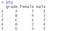
is a data box that doesn’t mean anything, but what you would expect, is the distribution of scores by sex.
Variables of the female and male is said above is contained in the variable name variable, female and male should be “gender” the variable values of the variables, the number of the following variable names (or attribute name) should be the “number”, we need to keep the original grade a list below, get rid of the female and male two columns, increase sex and count two columns, values with the original table corresponding to the up respectively, using the gather function:

gather(stu, gender, count,-grade)

The first parameter is the original data STU, the second and third parameters are key-value pairs (gender, number of people), and the fourth parameter is subtracting (remove the grade column, only the remaining two columns are transposed).

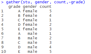
If you look at the two columns in the original table, they correspond like this:
(female, 5), (female, 4), (female, 1), (female, 2), (female, 3)
(male, 1), (male, 2), (male, 3), (male, 4), (male, 5),
The original variable name (attribute name) is used as the key and the variable value as the value.
Now we can continue with the normal statistical analysis.
separate()
Separate the data in a variable that contains two variables. (The name of an attribute “Gather” is a variable.)
Separate (), for example
Construct a new data box Stu2:

stu2<-data.frame(grade=c("A","B","C","D","E"), 
                 female_1=c(5, 4, 1, 2, 3), male_1=c(1, 2, 3, 4, 5),
                 female_2=c(4, 5, 1, 2, 3), male_2=c(0, 2, 3, 4, 6))

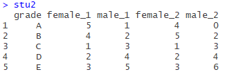
is similar to stU above, with 1 and 2 after sex denoting classes
So let’s just use the Gather function and transpose:

stu2_new<-gather(stu2,gender_class,count,-grade)

No, just like above, the result is as follows:

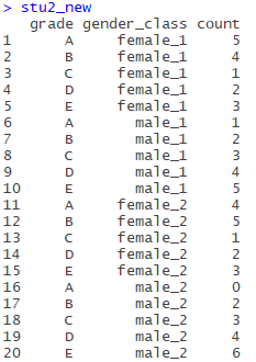
While this table is still not a standard two-dimensional table, we have found a column (gender_class) with values containing multiple attributes (variables), separated by separate(), which is used as follows:
Separate (Data, Col, into, SEP (= regular expression), remove =TRUE,convert = FALSE, extra = “warn”, Fill = “warn”…)
The first parameter puts the data box to be separated;
The second argument puts the column to be separated;
The third parameter is the column (which must be multiple) of the split variable, represented by a vector;
The fourth argument is a delimiter, denoted by a regular expression, or a number, denoted by which digit it is separated from (in the documentation:
If character, is interpreted as a regular expression. The default value is a regular expression that matches any sequence of non-alphanumeric values.
If numeric, interpreted as positions to split at. Positive values start at 1 at the far-left of the string; Negative value start at-1 at the far right of the string. The length of sep should be one less than into.)
The following parameters are not clear, you can see the documentation
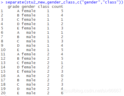
Now all we need to do is separate the gender_class column:

separate(stu2_new,gender_class,c("gender","class"))

Note that the third parameter is a vector, denoted by c(), and the fourth parameter should be “_”, omitted here (may be underlined is the default separator?).
The results are as follows:

spread()
Spread is used to extend the table to separate the values of a column (key-value pairs) into multiple columns.
spread(data, key, value, fill = NA, convert = FALSE, drop =TRUE, sep = NULL)
Key is the name of the original column (variable name), and value is what the value of those columns should be (which column of the original table should be filled).
So let’s go straight to the example
The spread (), for example
Construct data box Stu3:

name<-rep(c("Sally","Jeff","Roger","Karen","Brain"),c(2,2,2,2,2))
test<-rep(c("midterm","final"),5)
class1<-c("A","C",NA,NA,NA,NA,NA,NA,"B","B")
class2<-c(NA,NA,"D","E","C","A",NA,NA,NA,NA)
class3<-c("B","C",NA,NA,NA,NA,"C","C",NA,NA)
class4<-c(NA,NA,"A","C",NA,NA,"A","A",NA,NA)
class5<-c(NA,NA,NA,NA,"B","A",NA,NA,"A","C")
stu3<-data.frame(name,test,class1,class2,class3,class4,class5)


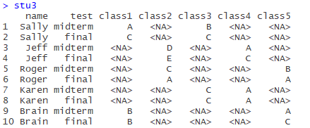
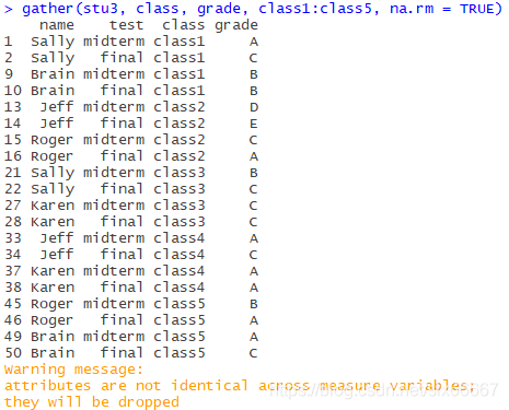
There are 5 courses in total. Each student chooses 2 courses and lists the mid-term and final grades.
Obviously, the original table is dirty data, and the header contains the variable (class1-5), so use the Gather function first. Note that there are many missing values, so you can use the na.rm=TRUE parameter above to automatically remove records with missing values (a record is a row) :

If I didn’t write na.rm=TRUE, it would look like this:
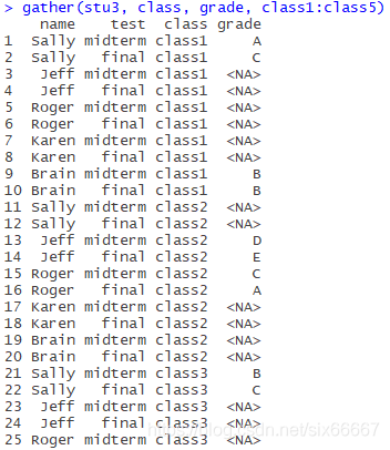
(Incomplete)
It is meaningless to analyze the “NA” score of students who have not selected courses, so records with missing values should be discarded in this case.
Now this table looks very neat, but everyone has four records, in which the values of test and grade are different for each course, the names and courses are the same, and most of the time, we need to carry out statistical analysis on mid-term and final scores respectively, so this table is not conducive to classification statistics.
The test is midterm and final with the spread function, and the values of these two columns are the results of the two courses I chose.
Again, the second argument is the column name of the column to be split, and the third argument is the column name of which column the value of the expanded column should come from in the original table.

stu3_new<-gather(stu3, class, grade, class1:class5, na.rm = TRUE)
spread(stu3_new,test,grade)

The results are as follows:

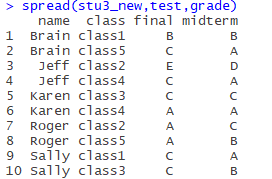
Now that you have a very neat table with only 10 pieces of data, it’s much easier to process.
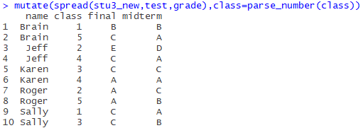
Finally, the class column is now a little redundant, and it’s a little more neat to just put Numbers in, use the parse_number() in the readr package to pull out the number(with the addition of dplyr’s mutate function), and let out the code:

install.packages("dplyr")
install.packages("readr")
library(readr)
library(dplyr)
mutate(spread(stu3_new,test,grade),class=parse_number(class))

Final results:

Isn’t neat very good-looking!! (* ╹ del ╹ *)

package R does not exist

This error is usually the result of not writing or incorrectly writing the package name in the source file. Note that this error is consistent with the package name in the Androidmanifest.xml.

ISLR reading notes (3) classification

Welcome to visit the personal homepage, the current traffic is too low, Baidu search can not say… Thank you for encouraging
reading notes. Instead of translating the full text, I plan to share the important knowledge points in the book with my own understanding, and attach the application of R language related functions at the end, as a summary of my recent learning in machine learning. If you don’t understand correctly, please correct me.

preface
ISLR, fully known as An Introduction to Statistical Learning with Applications in R, is a basic version of the Elements of Statistical Learning. The formula derivation in ISLR is not much, but mainly explains some commonly used methods in Statistical Learning and the application of relevant methods in R language. The ISLR doesn’t officially have the answers to the problem sets, but someone has created one, and you can learn from the ISLR answers
Chapter 4 Understanding
This chapter explains three methods of classification.
1. Logistic Regression(Logistic Regression)
2. Linear Discriminant Analysis
3. Quadratic Discriminant Analysis
The four categories are analyzed and compared one by one.
1.Logistic Regression
Formula:

The log (1 – p (x) p (x) = 0 + beta beta 1 x1 + beta 2 x2 +…

among them,

p(x)
Is the probability of belonging to a certain anomaly, is the final output,

Beta.
Is a parameter in Logistic Regression, and the optimal solution is generally obtained by the method of maximum likelihood. The general fitting curve is as follows:


Generally speaking, LOGICAL regression is suitable for the classification of two kinds of problems, and Discriminant Analysis is generally used for the classification of more than two kinds of problems.
2.Linear Discriminant Analysis
In fact, the discriminant method is to add the assumption that the model distribution follows the normal distribution on the basis of the original Bayesian theory. In the linear discriminant, it is assumed that the covariance of different variables is the same

The ellipse in the left figure is the normal distribution curve, and the boundary line intersected by two sides forms the classification boundary, while the real line in the right figure is the Bayesian estimation, which is the actual boundary line. It can be found that the accuracy of the linear discriminant method is still very good.
3.Quadratic Discriminant Analysis(Quadratic Discriminant)
The only difference between a quadratic discriminant and a linear discriminant is that you assume that the covariances of different variables are different, and that causes the dividing line to be curved on the graph, and you take the degrees of freedom from

p(p+1)/2
Increased to

Kp(p+1)/2
K is the number of variables. The effect of increased freedom can be seen in reading Notes (1).

The purple dotted line represents the actual boundary, the black dotted line represents the linear discriminant boundary, and the green solid line represents the quadratic discriminant boundary. It can be seen that the linear discriminant performs better when the boundary is linear; When the dividing line is nonlinear, the opposite is true.
4. To summarize
When the actual dividing line is linear, the linear discriminant performs better if the data is close to the normal distribution hypothesis, and the logistic regression performs better if the data is not close to the normal distribution hypothesis.
when the actual boundary line is nonlinear, the quadratic discriminant will be fitted. In other higher order or irregular cases, KNN performs well.
R language application
1. Import data and prepare

> library(ISLR)
> dim(Caravan)
[1] 5822   86
> attach(Caravan)
> summary(Purchase)
  No  Yes
5474  348

Since KNN is to be used later and distance is needed, the variables are normalized. The normalization program is just one sentence, and the normalization effect is shown in the following sentences.

> standardized.X = scale(Caravan[,-86])
> var(Caravan[,1])
[1] 165.0378
> var(Caravan[,2])
[1] 0.1647078
> var(standardized.X[,1])
[1] 1
> var(standardized.X[,2])
[1] 1

Establish test samples and training samples

> test = 1:1000
> train.X = standardized.X[-test,]
> test.X = standardized.X[test,]
> train.Y = Purchase[-test]
> test.Y = Purchase[test]

(c) Logistic Regression

> glm.fit = glm(Purchase~., data=Caravan, family = binomial, subset = -test)
Warning message:
glm.fit: fitted probabilities numerically 0 or 1 occurred
> glm.probs = predict(glm.fit, Caravan[test, ], type="response")
> glm.pred = rep("No", 1000)
> glm.pred[glm.probs>.5]="Yes"
> table(glm.pred, test.Y)
        test.Y
glm.pred  No Yes
     No  934  59
     Yes   7   0
> mean(glm.pred == test.Y)
[1] 0.934

3.Linear Discriminant Analysis

> library(MASS)
> lda.fit = lda(Purchase~.,data = Caravan, subset = -test)
> lda.pred = predict(lda.fit, Caravan[test,])
> lda.class = lda.pred$class
> table(lda.class, test.Y)
         test.Y
lda.class  No Yes
      No  933  55
      Yes   8   4
> mean(lda.class==test.Y)
[1] 0.937

4.Quadratic Discriminant Analysis(Quadratic Discriminant)

> qda.fit = qda(Purchase~.,data = Caravan, subset = -test)
Error in qda.default(x, grouping, ...) : rank deficiency in group Yes
> qda.fit = qda(Purchase~ABYSTAND+AINBOED,data = Caravan, subset = -test)

Found that direct training can cause errors… The two variables have been tried successfully. It seems that the dimension is too high, so far no solution has been found. Other applications are similar to LDA
5.KNN
parameter k can be selected by itself, and the input order of KNN function variables should be noted

> library(class)
> knn.pred = knn(train.X, test.X, train.Y,k=1)
> mean(test.Y==knn.pred)
[1] 0.882