Tag Archives: matlab

Matlab draw logarithmic coordinates!

In many engineering problems, some characteristics of data can be seen more clearly through logarithmic transformation of data. The curve of data points depicted in logarithmic coordinate system can directly represent logarithmic transformation.
There are two kinds of logarithmic transformation: double logarithmic transformation and single axis logarithmic transformation. Loglog function can be used to achieve the double log coordinate transformation, semilogx and Semilogy functions can be used to achieve the single axis log coordinate transformation.
Loglog (Y) means that the x and Y coordinates are logarithmic coordinates
Semilogx (Y) means that the x axis is a logarithmic coordinate system
Semilogy (…). That means that the Y-axis is a logarithmic coordinate system
So plotyy has two y axes, one on the left and one on the right
Example 1: Create a simple loglog with the square tag.
Solution: Enter a command
X = logspace (1, 2);
loglog(x,exp(x),’-s’)
Grid on % annotated grid
The produced figure is:

Example 2: Create a simple semi-logarithmic graph.
Solve input command:
x=0:.1:10;
semilogy(x,10.^x)
The produced figure is:

example 3: draw function graph, logarithmic graph and semilogarithmic graph of y=x^3.
Solution: Enter in the window:
x=[1:1:100];
Subplot (2,3,1);
plot(x,x.^3);
grid on;
title ‘plot-y=x^3’;

Subplot (2, 31);
loglog(x,x.^3);
grid on;
title ‘loglog-logy=3logx’;

Subplot (2 filling);
plotyy(x,x.^3,x,x);
grid on;
title ‘plotyy-y=x^3,logy=3logx’;

Subplot (2, 4);
semilogx(x,x.^3);
grid on;
title ‘semilogx-y=3logx’;

Subplot (2,3,5);
semilogy(x,x.^3);
grid on;
title ‘semilogy-logy=x^3’;
The produced figure is:

Empty Matrices, Scalars, and Vectors

Overview
Although matrices are two dimensional, they do not always appear to have a rectangular shape. A 1-by-8 matrix, for example, has two dimensions yet is linear. These matrices are described in the following sections:
The Empty Matrix An empty matrix has one or more dimensions that are equal to zero. A two-dimensional matrix with both dimensions equal to zero appears in the MATLAB^® application as []. The expression A = [] assigns a 0-by-0 empty matrix to A. Scalars A scalar is 1-by-1 and appears in MATLAB as a single real or complex number (e.g., 7, 583.62, -3.51, 5.46097e-14, 83+4i). Vectors A vector is 1-by-n or n-by-1, and appears in MATLAB as a row or column of real or complex numbers:

     Column Vector                 Row Vector

         53.2                  53.2 87.39 4-12i 43.9
         87.39
         4-12i
         43.9

The Empty Matrix
A matrix having at least one dimension equal to zero is called an empty matrix. The simplest empty matrix is 0-by-0 in size. Examples of more complex matrices are those of dimension 0-by-5 or 10-by-0.
To create a 0-by-0 matrix, use the square bracket operators with no value specified:

A = [];

whos A
  Name      Size            Bytes  Class     Attributes

  A         0x0                 0  double

You can create empty matrices (and arrays) of other sizes using the zeros, ones, rand, or eye functions. To create a 0-by-5 matrix, for example, use

A = zeros(0,5)
A =

  0×5 empty double matrix

Operating on an Empty Matrix

The basic model for empty matrices is that any operation that is defined for m-by-n matrices, and that produces a result whose dimension is some function of m and n, should still be allowed when m or n is zero. The size of the result of this operation is consistent with the size of the result generated when working with nonempty values, but instead is evaluated at zero.
For example, horizontal concatenation

C = [A B]

requires that A and B have the same number of rows. So if A is m-by-n and B is m-by-p, then C is m-by-(n+p). This is still true if m, n, or p is zero.
As with all matrices in MATLAB, you must follow the rules concerning compatible dimensions. In the following example, an attempt to add a 1-by-3 matrix to a 0-by-3 empty matrix results in an error:

[1 2 3] + ones(0,3)
Error using +
Matrix dimensions must agree.

Common Operations. The following operations return zero on an empty array:

A = [];
size(A), length(A), numel(A), any(A), sum(A)

These operations return a nonzero value on an empty array :

A = [];
ndims(A), isnumeric(A), isreal(A), isfloat(A), isempty(A), ...
   all(A), prod(A)

Using Empty Matrices in Relational Operations

You can use empty matrices in relational operations such as “equal to” (==) or “greater than” (>) as long as both operands have the same dimensions, or the nonempty operand is scalar. The result of any relational operation involving an empty matrix is the empty matrix. Even comparing an empty matrix for equality to itself does not return true, but instead yields an empty matrix:

x = ones(0,3);
y = x;

y == x
ans =

  0×3 empty logical array

Using Empty Matrices in Logical Operations

MATLAB has two distinct types of logical operators:
Short-circuit (&&, ||) — Used in testing multiple logical conditions (e.g., x >= 50 && x < 100) where each condition evaluates to a scalar true or false. Element-wise (&, |) — Performs a logical AND, OR, or NOT on each element of a matrix or array.
Short-circuit Operations. The rule for operands used in short-circuit operations is that each operand must be convertible to a logical scalar value. Because of this rule, empty matrices cannot be used in short-circuit logical operations. Such operations return an error.
The only exception is in the case where MATLAB can determine the result of a logical statement without having to evaluate the entire expression. This is true for the following two statements because the result of the entire statements are known by considering just the first term:

true || []
ans =

  logical

   1

false && []
ans =

  logical

   0

Element-wise Operations. Unlike the short-circuit operators, all element-wise operations on empty matrices are considered valid as long as the dimensions of the operands agree, or the nonempty operand is scalar. Element-wise operations on empty matrices always return an empty matrix:

true | []
ans =

  0×0 empty logical array

Note This behavior is consistent with the way MATLAB does scalar expansion with binary operators, wherein the nonscalar operand determines the size of the result.

Scalars
Any individual real or complex number is represented in MATLAB as a 1-by-1 matrix called a scalar value:

A = 5;

ndims(A)        % Check number of dimensions in A
ans =
     2

size(A)         % Check value of row and column dimensions
ans =
     1     1

Use the isscalar function to tell if a variable holds a scalar value:

isscalar(A)
ans =

  logical

   1

Vectors

Matrices with one dimension equal to one and the other greater than one are called vectors. Here is an example of a numeric vector:

A = [5.73 2-4i 9/7 25e3 .046 sqrt(32) 8j];

size(A)         % Check value of row and column dimensions
ans =
     1     7

You can construct a vector out of other vectors, as long as the critical dimensions agree. All components of a row vector must be scalars or other row vectors. Similarly, all components of a column vector must be scalars or other column vectors:

A = [29 43 77 9 21];
B = [0 46 11];

C = [A 5 ones(1,3) B]
C =
   29   43   77    9   21    5    1    1    1    0   46   11

Concatenating an empty matrix to a vector has no effect on the resulting vector. The empty matrix is ignored in this case:

A = [5.36; 7.01; []; 9.44]
A =
    5.3600
    7.0100
    9.4400

Use the isvector function to tell if a variable holds a vector:

isvector(A)
ans =

  logical

   1

How to express ln function in MATLAB?

LNX is log of x;

And log x is written as log base 10 of x.

Matlab delete row or col to delete the row or column of the matrix

In Matlab, we sometimes need to delete a row or a column in the matrix, which can be deleted by the following methods:

a = [
1 2 3
4 5 6
7 8 9];

a(2,:) = []; % Delete row 2
a(:,2) = []; % Delete col 2

Matlab — looking for peak function

Reproduced indicate the source: http://write.blog.csdn.net/postlist
Method one:

findpeaks function

PKS = findpeaks(data)

[PKS,locs] = findpeaks(data) — the number of peaks corresponding to PKS and locs

[…] = findpeaks(data,’minpeakheight’, MPH)– MPH sets the minimum peakheight

[…] = findpeaks(data,’minpeakdistance’, MPD)– MPD sets the minimum interval between two peaks

[…] = findpeaks(data,’threshold’,th)

[…] = findpeaks(data,’npeaks’,np)

[…] = findpeaks(data,’sortstr’, STR)

the command findpeaks is used to findpeaks of a vector that is greater than the value of two adjacent elements.
for example:
a=[1 3 2 5 6 8 5 3];
findpeaks(a),
returns 3 8
[v,l]= findbb2 (a),
returns
v=3 8
l=2 6
if a is a matrix, the values and locations of the peaks are listed in column search order.
For more information, see Help FindPeaks
Disadvantages:
You can only find the peak, you can’t find the trough.

Reproduced indicate the source: http://write.blog.csdn.net/postlist

Method 2:
IndMin=find(diff(sign(diff(data)))> 0) + 1;
IndMax=find(diff(sign(diff(data)))< 0) + 1;

where,
IndMin, data(IndMin) corresponds to the trough data
IndMax,data(IndMax) corresponds to the crest data

>> a=[1 3 2 5 6 8 5 3]

a =

     1     3     2     5     6     8     5     3

>> IndMax=find(diff(sign(diff(a)))<0)+1

IndMax =

     2     6

>> a(IndMax)

ans =

     3     8

>> IndMin=find(diff(sign(diff(a)))>0)+1

IndMin =

     3

>> a(IndMin)

ans =

     2

Reprint with reference to:
http://write.blog.csdn.net/postlist

What are the common clearing commands in MATLAB?

(If you need various versions of MATLAB software, you can leave a message and immediately reply when you see it.)
https://blog.csdn.net/weibo1230123/article/details/81016643
What are the common clear commands in MATLAB?

1.clc command: empty the command window.
2. CLF command: clear the current figure.
3. Close command: close the currently open figure graphical interface.
4. Clear: clear the variables in the workspace. 5. Exit command: exit MATLAB, and directly exit the software after execution.

The image operation of MATLAB — every detail operation of colorbar

Recently in the paper matlab generated height field, online search a lot, do a small summary of their own.

First, if you want to add colorbar to the generated image, you can do it in two ways:
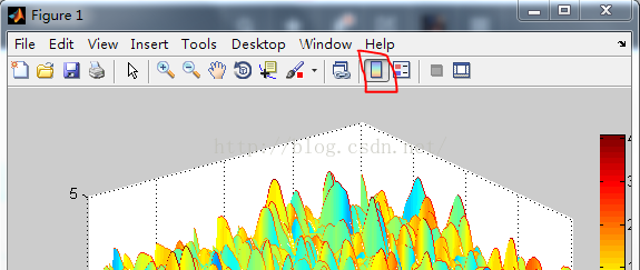
1: Insert — Colorbar in the menu bar of the generated Figure image, or click on the shortcut area at the top to add Colorbar, as shown below:

2: Directly from the command line

colorbar;

If you want to specify the location at will:

colorbar('position',[0.95 0.1 0.04 0.8]);

The data in square brackets refer to the x-coordinate, y-coordinate, width, and height of the colorbar bottom-left point. You can try to change the data and see what happens.

Second, sometimes the resulting colorbar is not what we want it to be. How can we arbitrarily adjust the range and position of the colorbar?

Here is a control method for a program statement:

1、set(a, 'CLim', [0 1]);
2、caxis([0,1]);

before colorbar, you can set its upper and lower limits, usually the second method is relatively simple!

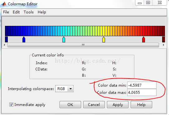
To adjust the value range of the colorbar, right-click on it and select Launch ColorMap Editor

So we want our colorbar to be as big, as long, as big, as wide as we want, and that’s pretty easy!
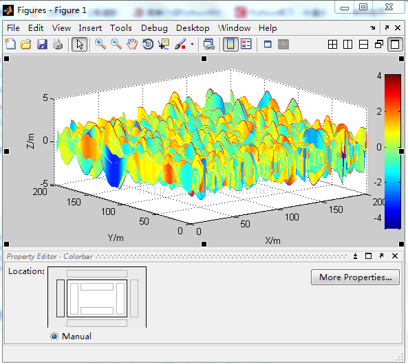
Click ColorBar, right-click — select Show Property Editor

Click on each of the small rectangles in Location to let our Colorbar position change.

We can even click colorbar in the image

Feel free to drag and resize.

The usage of Matlab function downsample

(I) Downsample
Reduce the sampling rate by an integer multiple

Continue Long Statements on Multiple Lines Matlab

This example shows how to continue a statement to the next line using ellipsis (...).

s = 1 - 1/2 + 1/3 - 1/4 + 1/5 ...
      - 1/6 + 1/7 - 1/8 + 1/9;

Build a long character string by concatenating shorter strings together:

mystring = ['Accelerating the pace of ' ... 
            'engineering and science'];

The start and end quotation marks for a string must appear on the same line. For example, this code returns an error, because each line contains only one quotation mark:

mystring = 'Accelerating the pace of ... 
            engineering and science'

An ellipsis outside a quoted string is equivalent to a space. For example,

x = [1.23...
4.56];

is the same as

x = [1.23 4.56];

How do I change the default background color of all FIGURE objects created in MATLAB

A list of factory-defined graphics settings that can be manipulated can be obtained by executing this command at the MATLAB prompt:

get(0,’Factory’)
To set the default color for all graphics objects, the ‘defaultfigurecolor’ property of the ROOT graphics object needs to be defined as follows:

set(0,’defaultfigurecolor’,[1 1 1])
Once the property is set, all succesive figures created will inherit this property from the ROOT graphics object.
More information on setting default color properties for handle graphics objects can be found here:

<http://www.mathworks.com/access/helpdesk/help/techdoc/index.html?/access/helpdesk/help/techdoc/creating_plots/f7-21465.html

The difference of four kinds of integer function (fix floor ceil round) in MATLAB

There are four integral functions in Matlab: Fix, floor, Ceil and Round. The specific application methods are as follows:

(1) fix
is rounded in the direction of zero
Such as
Fix (1.3) = 1
Fix (1.3) = 1;

(2) floor
is rounded in the direction of minus infinity (the maximum integer not exceeding x. (gaussian is rounded))
Such as
Floor (1.3) = 2
Floor (1.3) = 1;

(3) ceil
is rounded in the direction of positive infinity (the smallest integer greater than x)
Such as
The ceil (1.3) = 1
The ceil (1.3) = 2;

(4) round
rounded to the nearest integer
Such as
Round (1.3) = 1
Round (1.52) = 2
Round (1.3) = 1
Round (1.52) = 2

C ා use math.net Read. Mat file, file content is complex

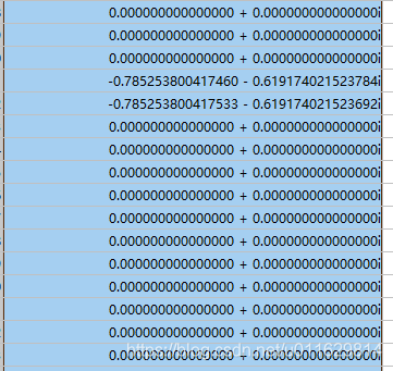
0. The project needs to read the complex file (.mat) generated by matlab simulation through C#, and then process it. The contents of the file are shown in the figure below:

1. Add DLL file: find Mathnet by NuGet manager, search mathnet.Numerics as shown in the figure below, install Mathnet.numerics;

2. Add references:

3. The following method can be used to read complex data.

ProgrammerAH

Programmer Guide, Tips and Tutorial