Author Archives: Robins

C# Bug Fixed InvalidCastException: Cannot cast from source type to destination type.

InvalidCastException: Cannot cast from source type to destination type.

Cannot convert from source type to target type.

The main reason for this problem is that there are errors in type conversion, one of which is not easy to detect is that there are errors when the parent class is cast to a subclass, that is, there may be errors when the transition is down in polymorphism

What is polymorphism: the pointer of the parent class points to the subclass and calls the method of the subclass

First let’s see where my code problem is, for your reference

Obviously, when I was in new tmphead, the pointer of the parent class did not point to the child class at all, so there would be no downward transformation.

We just need to change my code in this way to create a new subclass object..

How to Fix log4j2 warning: warn unable to identify org.fusesource.jansi.WindowsAnsiOutputStream

First knowledge of log4j2 and log4j

import org.apache.logging.log4j.LogManager;
import org.apache.logging.log4j.Logger;

public class Log4j2Test {
    public static void main(String[] args) {
        System.setProperty("log4j.skipJansi", "true");//2020-02-13 13:41:25,889 main WARN Unable to instantiate org.fusesource.jansi.WindowsAnsiOutputStream
//        Logger logger = LogManager.getLogger(LogManager.ROOT_LOGGER_NAME);
        Logger logger = LogManager.getLogger("mylog");
        logger.trace("trace level");
        logger.debug("debug level");
        logger.info("info level");
        logger.warn("warn level");
        logger.error("error level");
        logger.fatal("fatal level");
    }
}

If there is no log4j2.xml file in this project (recommended resources directory), the error will be reported and the running result will be

ERROR StatusLogger No log4j2 configuration file found. Using default configuration: logging only errors to the console.
14:12:28.891 [main] ERROR mylog - error level
14:12:28.894 [main] FATAL mylog - fatal level

When log4j2.xml is added to the resources directory, the content is

<?xml version="1.0" encoding="UTF-8"?>
<Configuration status="WARN">
    <properties>
        <property name="LOG_HOME">E:/logs</property>
        <property name="FILE_NAME">mylog</property>
        <property name="log.sql.level">info</property>
    </properties>


    <Appenders>
        <Console name="Console" target="SYSTEM_OUT">
            <PatternLayout pattern="%d{HH:mm:ss.SSS} [%t] %-5level %l - %msg%n" />
        </Console>

        <RollingRandomAccessFile name="RollingRandomAccessFile" fileName="${LOG_HOME}/${FILE_NAME}.log" filePattern="${LOG_HOME}/$${date:yyyy-MM}/${FILE_NAME}-%d{yyyy-MM-dd HH-mm}-%i.log">
            <PatternLayout pattern="%d{HH:mm:ss.SSS} [%t] %-5level %l - %msg%n"/>
            <Policies>
                <TimeBasedTriggeringPolicy interval="1"/>
                <SizeBasedTriggeringPolicy size="10 MB"/>
            </Policies>
            <DefaultRolloverStrategy max="20"/>
        </RollingRandomAccessFile>
    </Appenders>

    <Loggers>
        <Root level="warn">
            <AppenderRef ref="Console" />
            <AppenderRef ref="RollingRandomAccessFile" />
        </Root>

        <Logger name="com.dy.hbase2hbase" level="${log.sql.level}" additivity="false">
            <AppenderRef ref="Console" />
        </Logger>
        <Logger name="mylog" level="${log.sql.level}" additivity="false">
            <AppenderRef ref="Console" />
        </Logger>
    </Loggers>
</Configuration>

The location structure is shown in the figure

For the above error, just add the log4j.properties file in the resources directory, whose content is

log4j.rootLogger=info, stdout
log4j.appender.stdout=org.apache.log4j.ConsoleAppender
log4j.appender.stdout.layout=org.apache.log4j.PatternLayout
log4j.appender.stdout.layout.ConversionPattern=%d %p [%c] - %m%n
log4j.appender.logfile=org.apache.log4j.FileAppender
log4j.appender.logfile.File=target/spring.log
log4j.appender.logfile.layout=org.apache.log4j.PatternLayout
log4j.appender.logfile.layout.ConversionPattern=%d %p [%c] - %m%n
#1.Applications for consoles
#log4j.appender.CONSOLE = org.apache.log4j.ConsoleAppender 
#log4j.appender.Threshold = DEBUG 
#log4j.appender.CONSOLE.Target = System.out 
#log4j.appender.CONSOLE.layout = org.apache.log4j.PatternLayout 
#log4j.appender.CONSOLE.layout.ConversionPattern = [framework] % d - % c -%- 4r [ % t] %- 5p % c % x - % m % n 

##log4j.appender.CONSOLE.layout.ConversionPattern = [start] % d {DATE} [DATE] % n % p[PRIORITY] % n % x[NDC] % n % t[THREAD] n % c[CATEGORY] % n % m[MESSAGE] % n % n 

# 2.Applications for files
#log4j.appender.FILE = org.apache.log4j.FileAppender 
#log4j.appender.FILE.File = file.log 
#log4j.appender.FILE.Append = false 
#log4j.appender.FILE.layout = org.apache.log4j.PatternLayout 
#log4j.appender.FILE.layout.ConversionPattern = [framework] % d - % c -%- 4r [ % t] %- 5p % c % x - % m % n 

# Use this layout for LogFactor 5 analysis 

# 3.Applications for files
#log4j.appender.FILE = org.apache.log4j.FileAppender 
#log4j.appender.FILE.File = file.log 
#log4j.appender.FILE.Append = false 
#log4j.appender.FILE.layout = org.apache.log4j.PatternLayout 
#log4j.appender.FILE.layout.ConversionPattern = [framework] % d - % c -%- 4r [ % t] %- 5p % c % x - % m % n 

# Use this layout for LogFactor 5 analysis

And the project needs pom.xml by

        <!-- slf4j + log4j begin -->
        <dependency>
            <groupId>org.slf4j</groupId>
            <artifactId>slf4j-api</artifactId>
            <version>1.7.10</version>
        </dependency>

        <dependency>
            <groupId>org.apache.logging.log4j</groupId>
            <artifactId>log4j-api</artifactId>
            <version>${log4j.version}</version>
        </dependency>
        <dependency>
            <groupId>org.apache.logging.log4j</groupId>
            <artifactId>log4j-core</artifactId>
            <version>${log4j.version}</version>
        </dependency>
        <!-- log4j end-->

Python ValueError: only 2 non-keyword arguments accepted

Tiger input the following code on the problem, because there is no clear matrix format. Just add a box outside the matrix group. See the following for details.

source code

import time
import numpy as np

A = np.array([56.0, 0.0, 4.4, 68.0],
             [1.2, 104.0, 52.0, 8.0],
             [1.8, 135.0, 99.0, 0.9])

cal=A.sum(axis=0)
print(cal)

After modification

import time
import numpy as np

A = np.array([[56.0, 0.0, 4.4, 68.0],
             [1.2, 104.0, 52.0, 8.0],
             [1.8, 135.0, 99.0, 0.9]])

cal=A.sum(axis=0)
print(cal)

How to Fix KeyError: ‘plotly_domain’

1. Error description

E:\PycharmProjects\cdk\venv\Scripts\python.exe E:/PycharmProjects/cdk/venv/plotly/b.py
Traceback (most recent call last):
  File "E:/PycharmProjects/cdk/venv/plotly/b.py", line 14, in <module>
    py.iplot(data,filename='Histogram');
  File "E:\PycharmProjects\cdk\venv\lib\site-packages\plotly\plotly\plotly.py", line 170, in iplot
    return tools.embed(url, **embed_options)
  File "E:\PycharmProjects\cdk\venv\lib\site-packages\plotly\tools.py", line 404, in embed
    != session.get_session_config()['plotly_domain']):
KeyError: 'plotly_domain'

Process finished with exit code 1

2. Cause of error

import plotly;
import plotly.plotly as py;
import plotly.graph_objs as go;

plotly.tools.set_credentials_file(username='xxx',api_key='787889Pa0GMIkz1R3Z1BHy');

C = go.Bar(
    x = [1,2,3,4,5,6,7,8],
    y = [7889,5623,9856,1254,4878,5656,3562,7445]
)

data = [C];

py.iplot(data,filename='Histogram');

3. Solutions

When drawing graphics, you need to call the plot () method instead of the iPlot () method

import plotly;
import plotly.plotly as py;
import plotly.graph_objs as go;

plotly.tools.set_credentials_file(username='xxx',api_key='56895656GMIkz1R3Z1BHy');

C = go.Bar(
    x = [1,2,3,4,5,6,7,8],
    y = [7889,5623,9856,1254,4878,5656,3562,7445]
)

data = [C];

py.plot(data,filename='Histogram');

Python 3 urllib has no URLEncode attribute

Today, when practicing in pychar (I use python3), I found an attributeerror: module ‘urllib’ has no attribute ‘URLEncode’. Later, we found that the urllib structure of python2 and python3 is different.

Let me demonstrate it with python3 in pychar

Error example:

import urllib
import urllib.parse
wd =  {"wd":"video"}
print(urllib.urlencode(wd))

结果:

C:\Users\DELL\AppData\Local\Programs\Python\Python36-32\python.exe E:/untitled/Python_Test/urllib2Demo1.py
Traceback (most recent call last):
File “E:/untitled/Python_Test/urllib2Demo1.py”, line 5, in <module>
print(urllib.urlencode(wd))
AttributeError: module ‘urllib’ has no attribute ‘urlencode’
Process finished with exit code 1

Right Example

import urllib
import urllib.parse
wd =  {"wd":"video"}
print(urllib.parse.urlencode(wd))

result:

C:\Users\DELL\AppData\Local\Programs\Python\Python36-32\ python.exe E:/untitled/Python_ Test/urllib2Demo1.py
wd=%E4%BC%A0%E6%99%BA%E6%92%AD%E5%AE%A2

Process finished with exit code 0

So remember that the urllib library is different between python2 and python3.

Popularize the following knowledge points:

The difference of urllib library between python2 and python3

Urllib is a module provided by Python for operating URL.

In Python 2, there are urllib library and urllib2 library. In Python 3, urllib2 is merged into urllib library, which is often used when we crawl web pages.

After upgrading and merging, the location of packages in the module changes a lot.

Here are the common changes about urllib Library in python2 and python3:

    use import urllib2 in python2 — corresponding, import urllib2 will be used in python3 urllib.request , urllib.error Import urllib is used in python2 – Import urllib is used in python3 urllib.request , urllib.error , urllib.parse Use import urlparse in python2 — correspondingly, use import urlparse in python3 urllib.parse Use urllib2. Urlopen in python2 — corresponding, use urllib2. Urlopen in python3 urllib.request.urlopen Using in python2 urllib.urlencode ————Correspondingly, it will be used in Python 3 urllib.parse.urlencode Using in python2 urllib.quote ————Correspondingly, it will be used in Python 3 urllib.request.quote Using in python2 cookielib.Cookie Jar — corresponding, will be used in Python 3 http.CookieJar Use urllib2. Request in python2 — corresponding, use urllib2. Request in python3 urllib.request.Request

These are the common changes of urllib related modules from python2 to python3.

Warning when using numpy: runtimewarning: numpy.dtype size changed, may indicate binary incompatibility

You may encounter the following warnings when running Python programs after a new numpy installation:

/usr/local/lib/python2.7/dist-packages/scipy/linalg/basic.py:17: RuntimeWarning: numpy.dtype size changed, may indicate binary incompatibility. Expected 96, got 88
  from ._solve_toeplitz import levinson
/usr/local/lib/python2.7/dist-packages/scipy/linalg/__init__.py:207: RuntimeWarning: numpy.dtype size changed, may indicate binary incompatibility. Expected 96, got 88
  from ._decomp_update import *
/usr/local/lib/python2.7/dist-packages/scipy/special/__init__.py:640: RuntimeWarning: numpy.dtype size changed, may indicate binary incompatibility. Expected 96, got 88
  from ._ufuncs import *
/usr/local/lib/python2.7/dist-packages/scipy/special/_ellip_harm.py:7: RuntimeWarning: numpy.dtype size changed, may indicate binary incompatibility. Expected 96, got 88
  from ._ellip_harm_2 import _ellipsoid, _ellipsoid_norm
/usr/local/lib/python2.7/dist-packages/scipy/interpolate/_bsplines.py:10: RuntimeWarning: numpy.dtype size changed, may indicate binary incompatibility. Expected 96, got 88
  from . import _bspl
/usr/local/lib/python2.7/dist-packages/scipy/sparse/lil.py:19: RuntimeWarning: numpy.dtype size changed, may indicate binary incompatibility. Expected 96, got 88
  from . import _csparsetools
/usr/local/lib/python2.7/dist-packages/scipy/sparse/csgraph/__init__.py:165: RuntimeWarning: numpy.dtype size changed, may indicate binary incompatibility. Expected 96, got 88
  from ._shortest_path import shortest_path, floyd_warshall, dijkstra,\
/usr/local/lib/python2.7/dist-packages/scipy/sparse/csgraph/_validation.py:5: RuntimeWarning: numpy.dtype size changed, may indicate binary incompatibility. Expected 96, got 88
  from ._tools import csgraph_to_dense, csgraph_from_dense,\
/usr/local/lib/python2.7/dist-packages/scipy/sparse/csgraph/__init__.py:167: RuntimeWarning: numpy.dtype size changed, may indicate binary incompatibility. Expected 96, got 88
  from ._traversal import breadth_first_order, depth_first_order, \
/usr/local/lib/python2.7/dist-packages/scipy/sparse/csgraph/__init__.py:169: RuntimeWarning: numpy.dtype size changed, may indicate binary incompatibility. Expected 96, got 88
  from ._min_spanning_tree import minimum_spanning_tree
/usr/local/lib/python2.7/dist-packages/scipy/sparse/csgraph/__init__.py:170: RuntimeWarning: numpy.dtype size changed, may indicate binary incompatibility. Expected 96, got 88
  from ._reordering import reverse_cuthill_mckee, maximum_bipartite_matching, \
/usr/local/lib/python2.7/dist-packages/scipy/spatial/__init__.py:95: RuntimeWarning: numpy.dtype size changed, may indicate binary incompatibility. Expected 96, got 88
  from .ckdtree import *
/usr/local/lib/python2.7/dist-packages/scipy/spatial/__init__.py:96: RuntimeWarning: numpy.dtype size changed, may indicate binary incompatibility. Expected 96, got 88
  from .qhull import *
/usr/local/lib/python2.7/dist-packages/scipy/spatial/_spherical_voronoi.py:18: RuntimeWarning: numpy.dtype size changed, may indicate binary incompatibility. Expected 96, got 88
  from . import _voronoi
/usr/local/lib/python2.7/dist-packages/scipy/spatial/distance.py:122: RuntimeWarning: numpy.dtype size changed, may indicate binary incompatibility. Expected 96, got 88
  from . import _hausdorff

At this point, you can check the version of numpy below

python
>>> import numpy
>>> numpy.__version__

If version 1.15.0 or above is displayed, the warning is caused by too high numpy version. Downgrade numpy version, such as 1.14.5

sudo pip uninstall numpy
sudo pip install numpy==1.14.5

Android “handler” is abstract; can’t be identified solution

Today, when I use Android’s own refresh control, I need a handler for instance calls, but I report an error in my own instance calls
“handler” is abstract; can’t be identified
because there is an error in my import library. I use Android’s handler library instead of Java’s handle library
the solution is as follows
use “import” to import android.os.Handler ; ”Replace “import” java.util.logging .Handler;”

This can be solved, in addition to the reference to this blog

Cannot read property ‘this compilation’ of undefined appears in copy webpack plugin

Today, I want to copy the pictures of the company’s projects to build / images,

Direct installation

 npm install copy-webpack-plugin --save-dev

, using the latest official documentation

 new CopyPlugin({
      patterns: [
        { from: 'source', to: 'dest' },
        { from: 'other', to: 'public' },
      ],
    }),

However, it is always reported that cannot read property ‘this compilation’ of undefined

The results show that the webpack is “^ 1.13.2” because the company’s projects are older,

So you can reduce the copy webpack plugin version to below 5.0.0, and then use the old writing method

For example, “copy webpack plugin”: “^ 4.6.0”,

Deep learning: derivation of sigmoid function and loss function

1sigmoid function

1. Derivation from exponential function to sigmoid 2. Logarithm function and sigmoid 2. Sigmoid function 3. Neural network loss function derivation

1. Sigmoid function

Sigmoid function, i.e. S-shaped curve function, is as follows:
0

Function: F (z) = 11 + e − Z

Derivative: F ‘(z) = f (z) (1 − f (z))

The above is our common form. Although we know this form, we also know the calculation process. It’s not intuitive enough. Let’s analyze it.

1.1 from exponential function to sigmoid

First, let’s draw the basic graph of exponential function

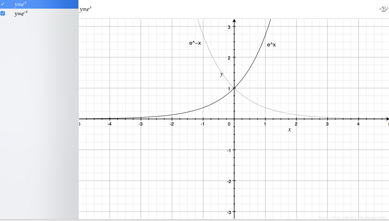
From the figure above, we get the following information: the exponential function passes (0,1) point, monotonically increasing / decreasing, and the definition field is

(−∞,+∞)

, the range is

(0,+∞)

Let’s take a look at the image of the sigmoid function
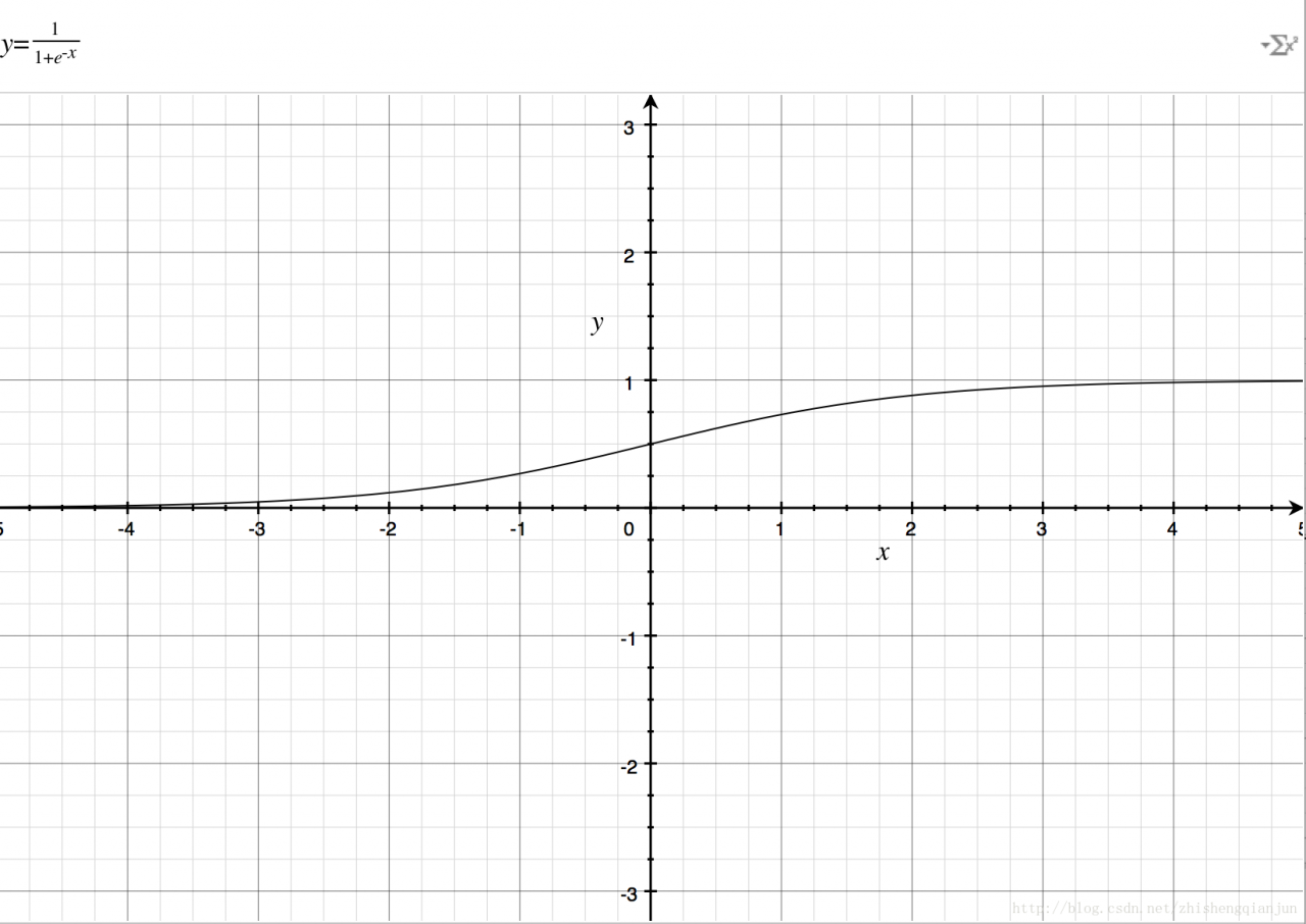
If you just

e−x

If you put it on the denominator, it’s the same as

ex

The image is the same, so add 1 to the denominator to get the image above. The domain of definition is

(−∞,+∞)

, the range is

(0,1)

Then there is a good feature, that is, no matter what

x

We can get the value between (0,1) for whatever it is;

1.2 logarithmic function and sigmoid

First, let’s look at the image of the logarithmic function

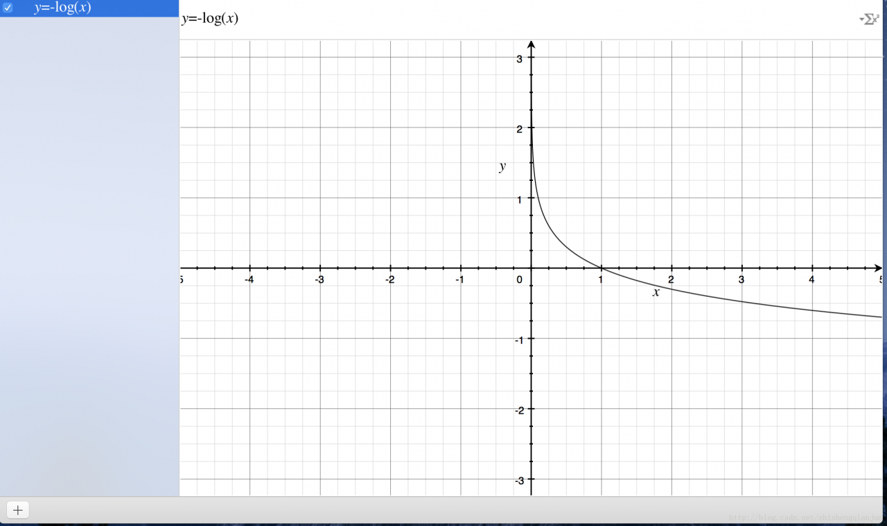
Logarithmic function of the image above, monotone decreasing, there is a better feature is in the

(0,1)

If we put the sigmoid function in front of us in the position of the independent variable, we will get the result

(0,1)

The image of the image;

How can we measure the difference between a result and the actual calculation? One idea is that if the result is closer, the difference will be smaller, otherwise, it will be larger. This function provides such an idea. If the calculated value is closer to 1, then it means that it is closer to the world result, otherwise, it is farther away. Therefore, this function can be used as the loss function of logistic regression classifier. If all the results are close to the result value, then The closer it is to 0. If the result is close to 0 after all the samples are calculated, it means that the calculated result is very close to the actual result.

2. Derivation of sigmoid function

The derivation process of sigmoid derivative is as follows:
0

f′(z)=(11+e−z)′=e−z(1+e−z)2=1+e−z−1(1+e−z)2=1(1+e−z)(1−1(1+e−z))=f(z)(1−f(z))

3. Derivation of neural network loss function

The loss function of neural network can be understood as a multi-level composite function, and the chain rule is used for derivation.

J(Θ)=−1m∑i=1m∑k=1K[y(i)klog((hΘ(x(i)))k)+(1−y(i)k)log(1−(hΘ(x(i)))k)]+λ2m∑l=1L−1∑i=1sl∑j=1sl+1(Θ(l)j,i)2

Let’s talk about the process of conventional derivation

e=(a+b)(b+1)

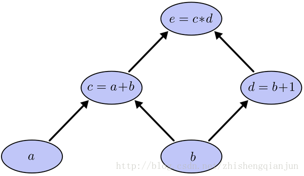
​ This is a simple composite function, as shown in the figure above. C is a function of a and E is a function of C. if we use the chain derivation rule to derive a and B respectively, then we will find out the derivative of e to C and C to a, multiply it, find out the derivative of e to C and D respectively, find out the derivative of C and D to B respectively, and then add it up, One of the problems is that in the process of solving, e calculates the derivative of C twice. If the equation is particularly complex, then the amount of calculation becomes very large. How can we only calculate the derivative once?

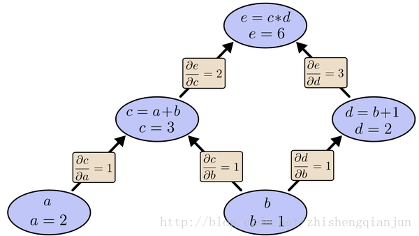
As shown in the figure above, we start from top to bottom, calculate the value of each cell, then calculate the partial derivative of each cell, and save it;

​ Next, continue to calculate the value of the sub unit, and save the partial derivatives of the sub unit; multiply all the partial derivatives of the path from the last sub unit to the root node, that is, the partial derivatives of the function to this variable. The essence of calculation is from top to bottom. When calculating, save the value and multiply it to the following unit, so that the partial derivatives of each path only need to be calculated once, from top to bottom All the partial derivatives are obtained by calculating them from top to bottom.

​ In fact, BP (back propagation algorithm) is calculated in this way. If there is a three-layer neural network with input layer, hidden layer and output layer, we can calculate the partial derivative of the weight of the loss function. It is a complex composite function. If we first calculate the partial derivative of the weight of the first layer, and then calculate the partial derivative of the weight of the second layer, we will find that there are some problems A lot of repeated calculation steps, like the example of simple function above, so, in order to avoid this kind of consumption, we use to find the partial derivative from the back to the front, find out the function value of each unit, find out the partial derivative of the corresponding unit, save it, multiply it all the time, and input the layer.

The following is a simple example to demonstrate the process of calculating partial derivative by back propagation

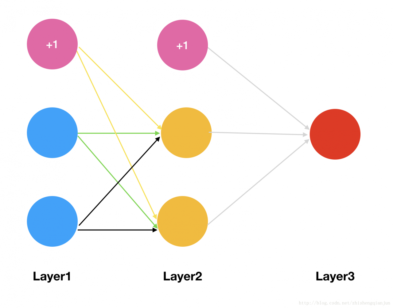
Then we will have two initial weight matrices:

θ1=[θ110θ120θ111θ121θ112θ122]θ2=[θ210θ211θ212]

We got the matrix above, and now we’re using

sigmoid

Function as the activation function to calculate the excitation of each layer of the network (assuming that we have only one sample, the input is

x1,x2,

The output is

y

);

The first level is input, and the incentive is the eigenvalue of the sample

a1=⎡⎣⎢⎢x0x1x2⎤⎦⎥⎥

x0

Is the bias term, which is 1

The second layer is the hidden layer. The excitation is obtained by multiplying the eigenvalue with the region, and then the sigmoid function is used to transform the region

a2

Before transformation

z2

z21z22z2a2a2=θ110∗x0+θ111∗x1+θ112∗x2=θ120∗x0+θ121∗x1+θ122∗x2=[z21z22]=sigmoid(z2)=⎡⎣⎢⎢⎢1a21a22⎤⎦⎥⎥⎥

In the above, we add a bias term at the end;

Next, the third layer is the output layer

z31z3a3a3=θ210∗a20+θ211∗a21+θ212∗a22=[z31]=sigmoid(z3)=[a31]

Because it is the output layer, there is no need to calculate further, so the bias term is not added;

The above calculation process, from input to output, is also called forward propagation.

Then, we write the formula of the loss function according to the loss function. Here, there is only one input and one output, so the loss function is relatively simple

Here, M = 1;
1

J(Θ)=−1m[y(i)klog((hΘ(x(i)))k)+(1−y(i)k)log(1−(hΘ(x(i)))k)]+λ2m∑l=1L−1∑i=1sl∑j=1sl+1(Θ(l)j,i)2=−1m[y∗log(a3)+(1−y)∗log(1−a3)]+λ2m∑l=1L−1∑i=1sl∑j=1sl+1(Θ(l)j,i)2

Note:

λ2m∑L−1l=1∑sli=1∑sl+1j=1(Θ(l)j,i)2

In fact, it is the sum of squares of all the weights. Generally, the one multiplied by the offset term will not be put in. This term is very simple. Ignore it for the time being, and do not write this term for the time being (this is regularization).

J(Θ)=−1m[y∗log(a3)+(1−y)∗log(1−a3)]

Then we get the above formula, and here we know if we want to ask for it

θ212

If we use the partial derivative of, we will find that this formula is actually a composite function,

y

It’s a constant. A3 is a constant

z3

Of

sigmoid

Function transformation, and

z3

then is

a2

Now that we have found where the weight is, we can start to find the partial derivative,

a3

finish writing sth.

s(z3)

Then, we get the following derivation:

∂J(Θ)∂θ212=−1m[y∗1s(z3)−(1−y)∗11−s(z3)]∗s(z3)∗(1−s(z3))∗a212=−1m[y∗(1−s(z3)−(1−y)∗s(z3)]∗a212=−1m[y−s(z3)]∗a212=1m[s(z3)−y]∗a212=1m[a3−y]∗a212

According to the above derivation, we can get the following formula:
1

∂J(Θ)∂θ210∂J(Θ)∂θ211=1m[a3−y]∗a210=1m[a3−y]∗a211

So, remember what I said earlier, we will seek the derivative from top to bottom and save the partial derivative of the current multiple subunits. According to the above formula, we know that the partial derivative of the second weight matrix can be obtained by

[a3−y]

It is obtained by multiplying the excitation of the previous layer of network and dividing it by the number of samples, so sometimes we call the difference as

δ3

Then, the partial derivatives of the second weight matrix are obtained by multiplying them in the form of matrix;

Now that we have obtained the partial derivatives of the second weight matrix, how can we find the partial derivatives of the first weight matrix?

For example, we’re going to

θ112

Partial derivation:
0

∂J(Θ)∂θ112=−1m[y∗1s(z3)−(1−y)∗11−s(z3)]∗s(z3)∗(1−s(z3))∗θ211∗s(z2)∗(1−s(z2))∗x2=−1m∗[a3−y]∗θ211∗s(z2)∗(1−s(z2))∗x2=−1m∗δ3∗θ211∗s(z2)∗(1−s(z2))∗x2

From the formula on the line, we can see that the derivative we saved can be directly multiplied. If there is a multi-layer network, in fact, the following process is the same as this one, so we get the formula:
if there is a multi-layer network, the following process is the same as this one

δ3δ2=a3−y=δ3∗(θ2)T∗s(z2)′

Because this network is three layers, so we can get all the partial derivatives. If it is multi-layer, the principle is the same. Multiply it continuously. Starting from the second formula, the following forms are the same.

Array initializer is not allowed here

Array initializer is not allowed here

The use of array is divided into declaration and initialization, which can be carried out simultaneously or separately

Int [] array; declaration

Array = New Int {element1, Element2, element3..}; initialization mode 1

Array = New Int [length]; initialization mode 2

There are two initialization methods for arrays

1、 Static initialization: the initial value of each array element is explicitly specified by the programmer during initialization;

    arrayName = new type[]{element1,element2,element3…}

2、 Dynamic initialization: when initializing, the programmer specifies the length of the array, and the system initializes the default value of each array element.

    arrayName = new type[length];

Note: do not use static initialization and dynamic initialization at the same time. In other words, do not specify the length of the array and divide each element of the array

The initial value is set.
 

Looking at the code today, we can see a simplified array initialization method, which belongs to the simplified version of static initialization, but there is something wrong with it

Int [] array = {1,2,3}; object [] obj = {}; this is OK

So I tried to write like this

Class member variables declare an array int [] elementdata, but it is not initialized;

Initialize it in the constructor, trying to write like this

Elementdata = {1,3,5}, so the above compilation error prompt appears

It seems that this simplified way of writing is not applicable here,

The use of arrays must be initialized

Suppose that elementdata = {1,3,5} does not generate new objects through new. Maybe the compiler thinks that it has been declared but not initialized

Therefore, it is recommended that the initialization is completed when the array is declared

Int [] elementdata = {1,3,5}; this is OK, declaration and assignment are done at the same time

Latex bold, italics

Latex bold, italics

Show upright text: textup {text}
Italians: textit {text}
slated: Italians: textsl {text}
show small upper case text: textsc {text}
medium weight: textmd {text}
bold command: textbf {text}
default: textnormal {text}