import mxnet as mx
from mxnet.gluon import nn
from mxnet import gluon,nd,autograd,init
from mxnet.gluon.data.vision import datasets,transforms
from IPython import display
import matplotlib.pyplot as plt
import time
import numpy as np

# download fashionMNIST data
fashion_train_data = datasets.FashionMNIST(train=True)
#get the infos of the img and the corrrsponding lable
images,labels = fashion_train_data[:]

#transforms swithc datas
transformer = transforms.Compose([
    transforms.ToTensor(),
    transforms.Normalize(0.13,0.31)])
#switch datas
fashion_data = fashion_train_data.transform_first(transformer)

#Set the size of the batch
batch_size = 256
# On windows system, please set num_workers to 0, otherwise it will cause thread error
train_data = gluon.data.DataLoader(fashion_data,batch_size=batch_size,shuffle=True,num_workers=0)

#Loading validation data
fashion_val_data = gluon.data.vision.FashionMNIST(train=False)
val_data = gluon.data.DataLoader(fashion_val_data.transform_first(transformer),
                                   batch_size=batch_size,num_workers=0)
#Define the GPU to be used, use GPU to accelerate training, if there are multiple GPUs, you can define more than one
gpu_devices = [mx.gpu(0)]
#define network structure
LeNet = nn.HybridSequential()
#Build a LeNet network structure
LeNet.add(
    nn.Conv2D(channels=6,kernel_size=5,activation="relu"),
    nn.MaxPool2D(pool_size=2,strides=2),
    nn.Conv2D(channels=16,kernel_size=3,activation="relu"),
    nn.MaxPool2D(pool_size=2,strides=2),
    nn.Flatten(),
    nn.Dense(120,activation="relu"),
    nn.Dense(84,activation="relu"),
    nn.Dense(10)
)
LeNet.hybridize()
#Initialize the weight parameters of the neural network, use GPU to accelerate the training
LeNet.collect_params().initialize(force_reinit=True,ctx=gpu_devices)
# Define softmax loss function
softmax_cross_entropy = gluon.loss.SoftmaxCrossEntropyLoss()
# set optimization algorithm, use stochastic gradient descent sgd algorithm, learning rate set to 0.1
trainer = gluon.trainer(LeNet.collect_params(), "sgd",{"learning_rate":0.1})
# Calculate the accuracy rate
def acc(output,label):
    return (output.argmax(axis=1) == label.astype("float32")).mean().asscalar()

#Set the number of iterations
epochs = 10
#training model
for epoch in range(epochs):
    train_loss,train_acc,val_acc = 0,0,0
    epoch_start_time = time.time()
    for data,label in train_data:
        #Use GPU to load data to accelerate training
        data_list = gluon.utils.split_and_load(data,gpu_devices)
        label_list = gluon.utils.split_and_load(label,gpu_devices)
        # forward propagation
        with autograd.record():
            #Get prediction results on multiple GPUs
            pred_Y = [LeNet(x) for x in data_list]
            #Calculate the loss of predicted values on multiple GPUs
            losses = [softmax_cross_entropy(pred_y,Y) for pred_y,Y in zip(pred_Y,label_list)]
        # backpropagation update parameters
        for l in losses:
            l.backward()
        trainer.step(batch_size)
        #Calculate the total loss on the training set
        train_loss += sum([l.sum().asscalar() for l in losses])
        # Calculate the accuracy on the training set
        train_acc += sum([acc(output_y,y) for output_y,y in zip(pred_Y,label_list)])

    for data,label in val_data:
        data_list = gluon.utils.split_and_load(data,ctx_list=gpu_devices)
        label_list = gluon.utils.split_and_load(label,ctx_list=gpu_devices)
        #Calculate the accuracy on the validation set
        val_acc += sum(acc(LeNet(val_X),val_Y) for val_X,val_Y in zip(data_list,label_list))

    print("epoch %d,loss:%.3f,train acc:%.3f,test acc:%.3f,in %.1f sec"%
          (epoch+1,train_loss/len(labels),train_acc/len(train_data),val_acc/len(val_data),time.time()-epoch_start_time))
#save
LeNet.export("lenet",epoch=1)

#loading the moudle files
LeNet = gluon.nn.SymbolBlock.imports("lenet-symbol.json",["data"],"lenet-0001.params")
Category Archives: Python
The Usage of Np.random.uniform()
np.random.uniform (low=0.0, high=1.0, size=None)
Function: random sampling from a uniform distribution [low, high]. Note that the definition field is left closed and right open, that is, it contains low but not high
Low: sampling lower bound, float type, default value is 0; high: sampling upper bound, float type, default value is 1; size: output sample number, int or tuple type, for example, size = (m, N, K), then output MNK samples, default value is 1. Return value: ndarray type, whose shape is consistent with the description in the parameter size.
The uniform () method randomly generates the next real number, which is in the range [x, y]
Evenly distributed, left closed, right open
np.random.uniform(1.75, 1, 100000000)
#output
array([1.25930467, 1.40160844, 1.53509096, ..., 1.57271193, 1.25317863,
       1.62040797])
Draw a picture to see the distribution
import matplotlib.pyplot as plt
# Generate a uniformly distributed random number
x1 = np.random.uniform(-1, 1, 100000000) # output the number of samples 100000000

# Draw a graph to see the distribution
# 1) Create a canvas
plt.figure(figuresize=(20, 8), dpi=100)

# 2) Plot the histogram
plt.hist(x1, 1000) # x represents the data to be used, bins represents the number of intervals to be divided

# 3) Display the image
plt.show()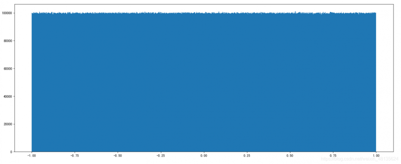
*
*
How does Python output colored fonts in the CMD command line window
Method 1
The output mode consists of three parts
\033 [font display mode; font color; font background color M ‘character’ \ 033 [0m]
Display mode: 0 (default), 1 (highlight), 22 (non BOLD), 4 (underline), 24 (non underline), 5 (flicker), 25 (non flicker), 7 (reverse display), 27 (non reverse display) font color: 30 (black), 31 (red), 32 (green), 33 (yellow), 34 (blue), 35 (magenta), 36 (cyan), 37 (white) font background color: 40 (black), 41 (red), 42 (green), 43 (yellow), 44 (blue), 45 (magenta), 46 (cyan), 47 (white)
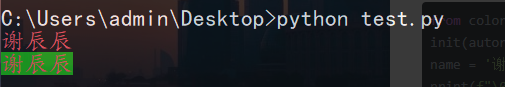
from colorama import init
init(autoreset=True)
name = '谢辰辰'
print(f"\033[0;31m{name}\033[0m")      #Output the red font
print(f"\033[0;31;42m{name}\033[0m") # Output the red font with green background color
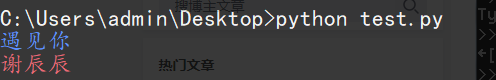
Method 2
Setting colors with fore
from colorama import init,Fore
init(autoreset=True)
print (Fore.BLUE+'遇见你')
print(Fore.RED+'谢辰辰')
Python_Syntax error: unexpected character after line continuation character
Python_ Syntax error: unexpected character after line continuation character
Reason: the content of the written file is incorrect and should be processed as a string
>>> import os
>>> os.makedirs(time_year+"\\"+time_month+"\\"+time_day)#where time_year, time_month, time_day are all variables with assigned values
>>> os.chdir(time_year\time_month\time_day)# The problem is here, it's not written correctly
  File "<stdin>", line 1
    os.chdir(time_year\time_month\time_day)
                                          ^
SyntaxError: unexpected character after line continuation character
This is OK: os.chdir (time_ year+”\\”+time_ month+”\\”+time_ day)
Refer to the writing method of creating directory in the first line
>>> os.chdir(time_year+"\\"+time_month+"\\"+time_day)#Correct
>>> with open(time_hours+".txt", "w+") as fp:#This method will go to the next step normally
...     fp.read()
...
Extracting TF-IDF keywords from text using Jieba
First install dependencies:
pip install -i https://pypi.tuna.tsinghua.edu.cn/simple/ jieba
Then use the following code:
import jieba.analyse


def tfidf_ana(content):
    content_s = "".join(content).strip()
    title_keys = jieba.analyse.extract_tags(content_s, topK=6, withWeight=False)  # topK is the number of keywords expected to be obtained
    title_keys = ','.join(title_keys)
    return title_keys


# begin to test
data = tfidf_ana("2019年,复杂的外部环境、全球经济放缓的较大可能性,叠加中国经济前期不利因素的累积效应,经济下行"
                 "压力进一步凸显,但是变中危和机同生共存,紧扣重要战略机遇新内涵,做好“六稳”工作,变压力为加快推动"
                 "经济高质量发展的动力。一是进一步发展好对外贸易关系,推进新全球化,以经贸关系为主线稳定外部环境。"
                 "稳妥应对外部经济环境变化,稳步发展“一带一路”贸易畅通,积极参与全球经济和贸易治理体系变革与发展,"
                 "坚持维护WTO的多边机制,维护中国在外贸中的合理权益和地位。二是稳妥处置地方政府债务风险和衍生金融风险。"
                 "为地方政府“开前门、堵后门”,辅以金融政策支持,为之构建合理的债务处置出口;合理划分中央和地方各级政府的财权、"
                 "事权,使地方政府的事权和财权相匹配,并有资源能够化解已有的债务问题,使之成为中国经济发展的助推器,而非风险源。"
                 "三是加快经济的深化改革和扩大开放。我国经济韧性强健,产业门类齐全,人员技能熟练,经济纵深宽广,抗风险能力强大,"
                 "加快经济的深化改革和扩大开放,深化国资国企、财税金融、土地、市场准入、社会管理等领域改革,推动体制机制创新,"
                 "不仅能进一步激发全社会的发展活力,为实现“六稳”目标打下坚实的基础,还能吸引中国经济对国际社会的吸引力,"
                 "形成互惠互利,提升中国应对全球经济衰退风险的能力,提高中国在推进新型全球化进程中的权益。
print(data)
Implementation of Kalman Filter in Python
Kalman filtering
In learning the principle of Kalman filtering, I hope to deepen the understanding of the formula and principle through python.
Take notes
import numpy as np
import math
import matplotlib.pyplot as plt

'''
    dynam_params:The dimensions of the state space.
    measure_params: the dimension of the measure value;
    control_params: the dimension of the control vector, default is 0.
'''
class Kalman(object):
    '''
        INIT KALMAN
    '''
    def __init__(self, dynam_params, measure_params,control_params = 0,type = np.float32):
        self.dynam_params = dynam_params
        self.measure_params = measure_params
        self.control_params = control_params
        # self

        ### The following should all be able to determine the dimension based on the input dimension value
        if(control_params ! = 0):
            self.controlMatrix = np.mat(np.zeros((dynam_params, control_params)),type) # control matrix
        else:
            self.controlMatrix = None
        self.errorCovPost =  np.mat(np.zeros((dynam_params, dynam_params)),type) # P_K
        self.errorCovPre =  np.mat(np.zeros((dynam_params, dynam_params)),type) # P_k-1
        self.gain =  np.mat(np.zeros((dynam_params, measure_params)),type) # K

        self.measurementMatrix =  np.mat(np.zeros((measure_params, dynam_params)),type)
        self.measurementNoiseCov =  np.mat(np.zeros((measure_params, measure_params)),type)
        self.processNoiseCov =  np.mat(np.zeros((dynam_params, dynam_params)),type)
        self.transitionMatrix =  np.mat(np.zeros((dynam_params, dynam_params)),type)

        self.statePost =  np.array(np.zeros((dynam_params, 1)),type)
        self.statePre =  np.array(np.zeros((dynam_params, 1)),type)

        # The diagonal is initialized to 1
        ## np.diag_indices returns the index of the main diagonal as a tuple
        ### F state transfer matrix diagonal initialized to 1
        row,col = np.diag_indices(self.transitionMatrix.shape[0])
        self.transitionMatrix[row,col] = np.array(np.ones(self.transitionMatrix.shape[0]))
        ### R measure noise Diagonal initialized to 1
        row,col = np.diag_indices(self.measurementNoiseCov.shape[0])
        self.measurementNoiseCov[row,col] = np.array(np.ones(self.measurementNoiseCov.shape[0]))
        ### Q Process noise Diagonal initialized to 1
        row,col = np.diag_indices(self.processNoiseCov.shape[0])
        self.processNoiseCov[row,col] = np.array(np.ones(self.processNoiseCov.shape[0]))

    def predict(self,control_vector = None):
        '''
            PREDICT
        '''
        # Predicted value
        F = self.transitionMatrix
        x_update = self.statePost
        B = self.controlMatrix

        if(self.control_params == 0):
            x_predict = F * x_update
        else:
            x_predict = F * x_update + B * control_vector
        self.statePre = x_predict

        # P_k
        P_k_minus = self.errorCovPost
        Q = self.processNoiseCov
        self.errorCovPre = F * P_k_minus * F.T + Q

        self.statePost = self.statePre
        self.errorCovPost = self.errorCovPre
        return x_predict

    def correct(self,mes):
        '''
            CORRECT
        '''
        # K update
        K = self.gain
        P_k = self.errorCovPost
        H = self.transitionMatrix
        R = self.measurementNoiseCov
        K = P_k * H.T * np.linalg.inv(H * P_k * H.T + R)
        self.gain = K

        # Calculate the estimated value of State
        x_predict = self.statePre
        x_update = x_predict +  K * (mes - H * x_predict)
        self.statePost = x_update

        # P_k update
        P_pre = self.errorCovPre
        P_k_post = P_pre - K * H * P_pre
        self.errorCovPost = P_k_post
        return x_update

if __name__ == '__main__':

    pos = np.array([
        [10,    50],
        [12,    49],
        [11,    52],
        [13,    52.2],
        [12.9,  50]], np.float32)
    kalman = Kalman(2,2)
    kalman.measurementMatrix = np.mat([[1,0],[0,1]],np.float32)
    kalman.transitionMatrix = np.mat([[1,0],[0,1]], np.float32)
    kalman.processNoiseCov = np.mat([[1,0],[0,1]], np.float32) * 1e-4
    kalman.measurementNoiseCov = np.mat([[1,0],[0,1]], np.float32) * 1e-4
    kalman.statePre =  np.mat([[6],[6]],np.float32)
   #kalman.statePre =  np.mat([[6],[6]],np.float32)
    for i in range(len(pos)):
        mes = np.reshape(pos[i,:],(2,1))
        y = kalman.predict()

        print("before correct mes",mes[0],mes[1])
        x = kalman.correct(mes)
        print (kalman.statePost[0],kalman.statePost[1])
        print (kalman.statePre[0],kalman.statePre[1])
        print ('measurement:\t',mes[0],mes[1])
        print ('correct:\t',x[0],x[1])
        print ('predict:\t',y[0],y[1])
        print ('='*30)
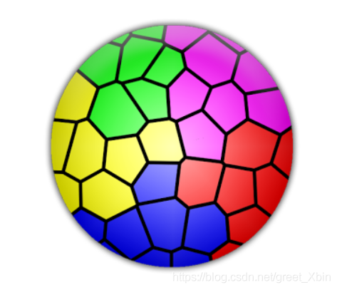
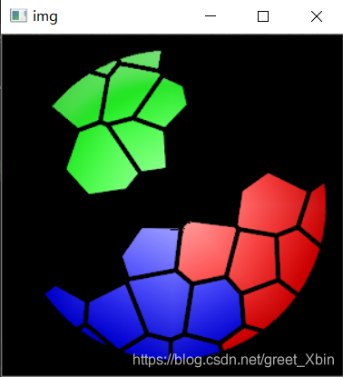
CV: How to extracts the part of the picture with the specified color
CV extracts the part of the picture with the specified color
How to extract the red, blue and green colors of the image below?
1. Import the library first
import cv2
import numpy as np
2. Read picture
The conversion between BGR and HSV uses CV2. Color_ BGR2HSV
img = cv2.imread("3.png")
hsv=cv2.cvtColor(img,cv2.COLOR_BGR2HSV)#HSV空间
(in HSV space, h is color/chroma, value range [0179], s is saturation, value range [0255], V is brightness, value range [0255].)
3. The threshold values of three colors are set and extracted
cv2.inRange(src, lowerb, upperb[, dst]) → dst
SRC – first input array. Input matrix (image)
lowerb – inclusive lower boundary array or a scalar. Lower threshold
upperrb – inclusive upper boundary array or a scalar. Upper threshold
DST – output array of the same size as SRC and CV_ 8U type. Output the same matrix as Src
lower_blue=np.array([110,100,100])#blue
upper_blue=np.array([130,255,255])

lower_green=np.array([60,100,100])#green
upper_green=np.array([70,255,255])

lower_red=np.array([0,100,100])#red
upper_red=np.array([10,255,255])

red_mask=cv2.inRange(hsv,lower_red,upper_red)
blue_mask=cv2.inRange(hsv,lower_blue,upper_blue)
green_mask=cv2.inRange(hsv,lower_green,upper_green)
4. Process the original image
red=cv2.bitwise_and(img,img,mask=red_mask)
green=cv2.bitwise_and(img,img,mask=green_mask)
blue=cv2.bitwise_and(img,img,mask=blue_mask)

res=green+red+blue
cv2.bitwise_ And() function is used to “and” binary data, that is, to binary “and” each pixel value of image (gray image or color image), 1 & amp; 1 = 1, 1 & amp; 0 = 0, 0 & amp; 1 = 0, 0 & amp; 0 = 0.
5. Output display
cv2.imshow('img',res)
cv2.waitKey(0)
cv2.destroyAllWindows()
6. Results display

All code packed
import cv2
import numpy as np


img = cv2.imread("3.png")
hsv=cv2.cvtColor(img,cv2.COLOR_BGR2HSV)

lower_blue=np.array([110,100,100])#blue
upper_blue=np.array([130,255,255])

lower_green=np.array([60,100,100])#green
upper_green=np.array([70,255,255])

lower_red=np.array([0,100,100])#red
upper_red=np.array([10,255,255])

red_mask=cv2.inRange(hsv,lower_red,upper_red)
blue_mask=cv2.inRange(hsv,lower_blue,upper_blue)
green_mask=cv2.inRange(hsv,lower_green,upper_green)

red=cv2.bitwise_and(img,img,mask=red_mask)
green=cv2.bitwise_and(img,img,mask=green_mask)
blue=cv2.bitwise_and(img,img,mask=blue_mask)

res=green+red+blue

cv2.imshow('img',res)
cv2.waitKey(0)

cv2.destroyAllWindows()
Command “/usr/bin/python -u -c “import setuptools, tokenize;__file__=‘/tmp/pip-cus9V0-build/setup.py
Command “/usr/bin/python -u -c “import setuptools, tokenize;file=’/tmp/pip-cus9V0-build/setup.py’;f=getattr(tokenize, ‘open’, open)(file);code=f.read().replace(’\r\n’, ‘\n’);f.close();exec(compile(code, file, ‘exec’))” install –record /tmp/pip-Ebvaxk-record/install-record.txt –single-version-externally-managed –compile” failed with error code 1 in /tmp/pip-cus9V0-build/
Solution:
ubuntu
apt-get install python-dev
cents
yum install python-devel
It should be the lack of Python dev dependency when running Python lzop
[resolution] str.contains() problem] valueerror: cannot index with vector containing Na/Nan values
Problem description;
when using dataframe, perform the following operations:
df[df.line.str.contains('G')]
The purpose is to find out all the lines in the line column of DF that contain the character ‘g’
---------------------------------------------------------------------------
ValueError                                Traceback (most recent call last)
<ipython-input-3-10f8503f73f2> in <module>()
---->  df.line.str.contains('G')

D:\Anaconda3\lib\site-packages\pandas\core\frame.py in __getitem__(self, key)
   2983
   2984         # Do we have a (boolean) 1d indexer?
-> 2985         if com.is_bool_indexer(key):
   2986             return self._getitem_bool_array(key)
   2987

D:\Anaconda3\lib\site-packages\pandas\core\common.py in is_bool_indexer(key)
    128             if not lib.is_bool_array(key):
    129                 if isna(key).any():
--> 130                     raise ValueError(na_msg)
    131                 return False
    132             return True

ValueError: cannot index with vector containing NA / NaN values
Obviously, it means that there are Na or Nan values in the line column, so Baidu has a lot of methods on the Internet to teach you how to delete the Na / Nan values in the line column.
However, deleting the row containing Na / Nan value in the line column still can’t solve the problem!! What shall I do?
Solution:
it’s very simple. In fact, it’s very likely that the element formats in the line column are not all STR formats, and there may be int formats, etc.
so you just need to unify the format of the line column into STR format!
The operation is as follows:
df['line'] = df['line'].apply(str) #Change the format of the line column to str

df[df.line.str.contains('G')] #Execute your corresponding statement
solve the problem!!
Autograd error in Python: runtimeerror: grad can be implicitly created only for scalar outputs
preface
Scalar is a tensor of order 0 (a number), which is 1 * 1;
vector is a tensor of order 1, which is 1 * n;
tensor can give the relationship between all coordinates, which is n * n.
So it is usually said that tensor (n * n) is reshaped into vector (1 * n). In fact, there is no big change in the reshaping process.
import torch
x=torch.ones(2,2,requires_grad=True)
print(x)
y=x+2
print(y)
#If a tensor is not created by the user, it has the grad_fn attribute. The grad_fn attribute holds a reference to the Function that created the tensor
print(y.grad_fn)
y.backward()
print(x.grad)
Running results
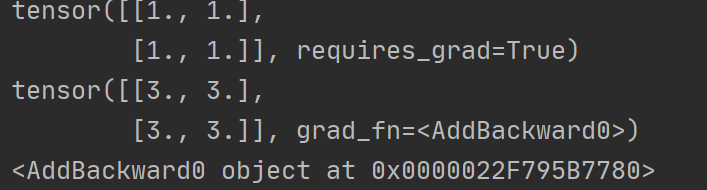
You can see that y is a tensor, which cannot use backward (), and needs to be converted to scalar,
Of course, tensor is also OK, that is, you need to change a code:
z.backward( torch.ones_ like(x))
Our return value is not a scalar, so we need to input a tensor of the same size as the parameter. Here we use ones_ The like function generates a tensor from X. In my opinion, because we want to obtain the derivative of X, the function y must be a value obtained, that is, a scalar. Then we start to find the partial derivatives of X and y, respectively.
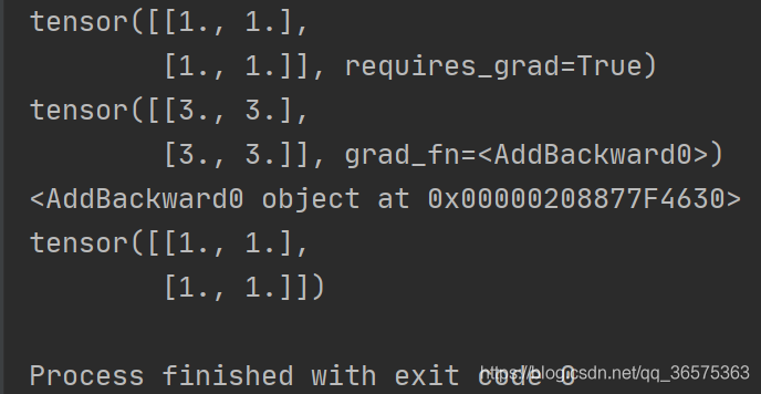
After modification
import torch
x=torch.ones(2,2,requires_grad=True)
print(x)
y=x+2
print(y)
#If a tensor is not created by the user, it has the grad_fn attribute. The grad_fn attribute holds a reference to the Function that created the tensor
print(y.grad_fn)
y.backward(torch.ones_like(x))
print(x.grad)
Running results
numpy.AxisError: axis 1 is out of bounds for array of dimension 1
Original address
The error occurred during the execution of np.concatenate (, axis = 1) when
When I want to pile up two one-dimensional data, that is
# Pre
a = [1,2,3]
b = [4,5,6]
# New
[[1,2,3],
[4,5,6]]
use np.concatenate ((a,b),axis=1)
This is because both a and B are one-dimensional data with only one dimension, that is, axis = 0, and there is no axis = 1
I found two solutions
np.vstack ((A,B))
A and B can be stacked vertically
print(np.vstack((a,b)))	# Note that the parameter passed is '(a,b)'
# [[1 2 3]
#  [4 5 6]]
The fly in the ointment is that this method can only pass two vectors to stack
np.newaxis + np.concatenate ()
Newaxis, as the name suggests, is a new axis. The usage is as follows
a = a[np.newaxis,:]	# Where ':' represents all dimensions (here 3), the shape of a becomes (1, 3), which is now two-dimensional
# [[1 2 3]]
b = b[np.newaxis,:]
# [[4 5 6]]
At this time, I can pile up two (1, 3) vectors into a matrix of (1 * 2, 3) = (2, 3). Note that axis = 0 should be used, that is, the first dimension
print(np.concatenate((a,b),axis=0))
# [[1 2 3]
#  [4 5 6]]
relevant
Numpy: matrix merging
Attr in wxPython= wx.grid.GridCellAttr() error reporting
Question:
wx._ core.wxAssertionError : C++ assertion “m_ count > 0” failed at … \src\common\ object.cpp (352) in wxRefCounter::DecRef(): invalid ref data count
Causes of the problem:
        attr = wx.grid.GridCellAttr()
        for i in range(len(lis)):
            editor = wx.grid.GridCellBoolEditor()
            self.SetCellEditor(i + 1, 0, editor)
            self.SetCellRenderer(i + 1, 0, wx.grid.GridCellBoolRenderer())
            for j in range(len(lis[i])):
                self.SetCellValue(i + 1, j + 1, lis[i][j])
                attr.SetReadOnly()
                self.SetAttr(i + 1, j + 1, attr)
Solution 1:
        #attr = wx.grid.GridCellAttr() #Modify the part
        for i in range(len(list1)):
          attr = wx.grid.GridCellAttr()#Modify the part
          self.SetCellValue(i + 1, j + 1, list1[i][j])
          attr.SetReadOnly()
          self.SetAttr(i + 1, j + 1, attr)
Solution 2:
        attr = wx.grid.GridCellAttr()
        for j in range(len(list1[i])):
              self.SetCellValue(i + 1, j + 1, list1[i][j])
              attr.SetReadOnly()
              atttr.IncRef()#Modify the part;this will leak the GridCellAttr, because the destructor is not called
              self.SetAttr(i + 1, j + 1, attr)