1sigmoid function
1. Derivation from exponential function to sigmoid 2. Logarithm function and sigmoid 2. Sigmoid function 3. Neural network loss function derivation
1. Sigmoid function
Sigmoid function, i.e. S-shaped curve function, is as follows:
0
Function: F (z) = 11 + e − Z
Derivative: F ‘(z) = f (z) (1 − f (z))
The above is our common form. Although we know this form, we also know the calculation process. It’s not intuitive enough. Let’s analyze it.
1.1 from exponential function to sigmoid
First, let’s draw the basic graph of exponential function
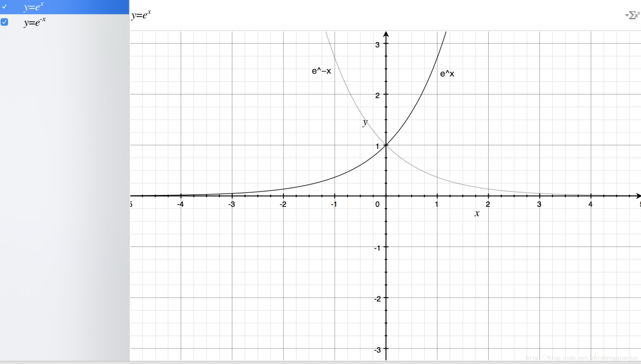
From the figure above, we get the following information: the exponential function passes (0,1) point, monotonically increasing / decreasing, and the definition field is
(−∞,+∞)
, the range is
(0,+∞)
Let’s take a look at the image of the sigmoid function
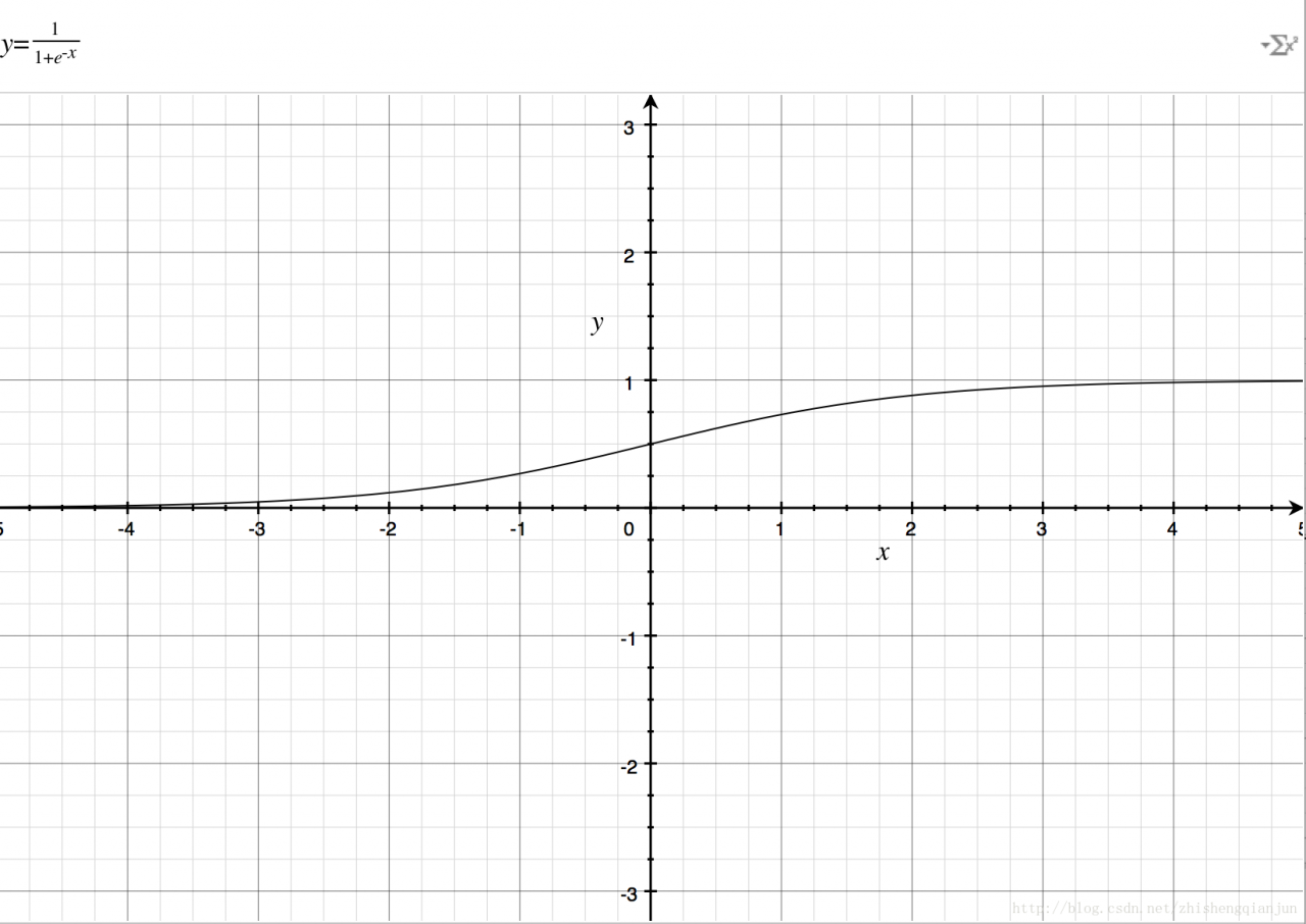
If you just
e−x
If you put it on the denominator, it’s the same as
ex
The image is the same, so add 1 to the denominator to get the image above. The domain of definition is
(−∞,+∞)
, the range is
(0,1)
Then there is a good feature, that is, no matter what
x
We can get the value between (0,1) for whatever it is;
1.2 logarithmic function and sigmoid
First, let’s look at the image of the logarithmic function
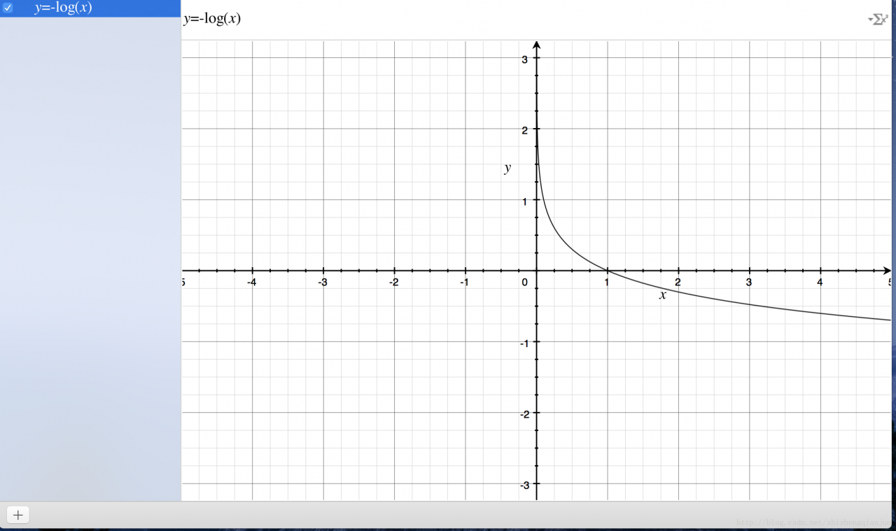
Logarithmic function of the image above, monotone decreasing, there is a better feature is in the
(0,1)
If we put the sigmoid function in front of us in the position of the independent variable, we will get the result
(0,1)
The image of the image;
How can we measure the difference between a result and the actual calculation? One idea is that if the result is closer, the difference will be smaller, otherwise, it will be larger. This function provides such an idea. If the calculated value is closer to 1, then it means that it is closer to the world result, otherwise, it is farther away. Therefore, this function can be used as the loss function of logistic regression classifier. If all the results are close to the result value, then The closer it is to 0. If the result is close to 0 after all the samples are calculated, it means that the calculated result is very close to the actual result.
2. Derivation of sigmoid function
The derivation process of sigmoid derivative is as follows:
0
f′(z)=(11+e−z)′=e−z(1+e−z)2=1+e−z−1(1+e−z)2=1(1+e−z)(1−1(1+e−z))=f(z)(1−f(z))
3. Derivation of neural network loss function
The loss function of neural network can be understood as a multi-level composite function, and the chain rule is used for derivation.
J(Θ)=−1m∑i=1m∑k=1K[y(i)klog((hΘ(x(i)))k)+(1−y(i)k)log(1−(hΘ(x(i)))k)]+λ2m∑l=1L−1∑i=1sl∑j=1sl+1(Θ(l)j,i)2
Let’s talk about the process of conventional derivation
e=(a+b)(b+1)
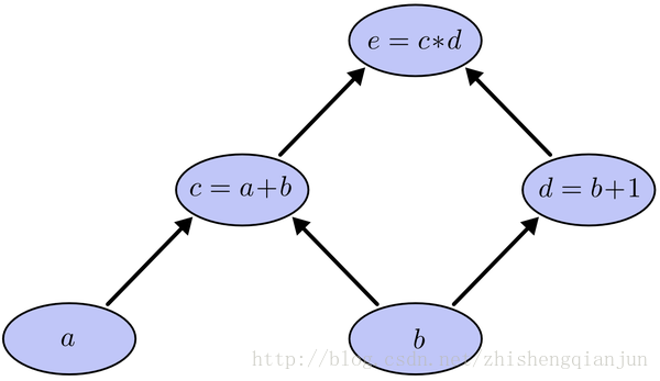
This is a simple composite function, as shown in the figure above. C is a function of a and E is a function of C. if we use the chain derivation rule to derive a and B respectively, then we will find out the derivative of e to C and C to a, multiply it, find out the derivative of e to C and D respectively, find out the derivative of C and D to B respectively, and then add it up, One of the problems is that in the process of solving, e calculates the derivative of C twice. If the equation is particularly complex, then the amount of calculation becomes very large. How can we only calculate the derivative once?
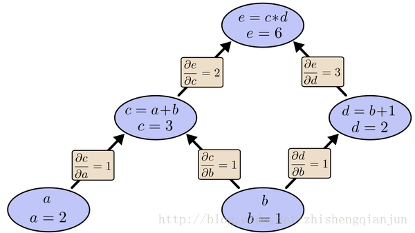
As shown in the figure above, we start from top to bottom, calculate the value of each cell, then calculate the partial derivative of each cell, and save it;
Next, continue to calculate the value of the sub unit, and save the partial derivatives of the sub unit; multiply all the partial derivatives of the path from the last sub unit to the root node, that is, the partial derivatives of the function to this variable. The essence of calculation is from top to bottom. When calculating, save the value and multiply it to the following unit, so that the partial derivatives of each path only need to be calculated once, from top to bottom All the partial derivatives are obtained by calculating them from top to bottom.
In fact, BP (back propagation algorithm) is calculated in this way. If there is a three-layer neural network with input layer, hidden layer and output layer, we can calculate the partial derivative of the weight of the loss function. It is a complex composite function. If we first calculate the partial derivative of the weight of the first layer, and then calculate the partial derivative of the weight of the second layer, we will find that there are some problems A lot of repeated calculation steps, like the example of simple function above, so, in order to avoid this kind of consumption, we use to find the partial derivative from the back to the front, find out the function value of each unit, find out the partial derivative of the corresponding unit, save it, multiply it all the time, and input the layer.
The following is a simple example to demonstrate the process of calculating partial derivative by back propagation
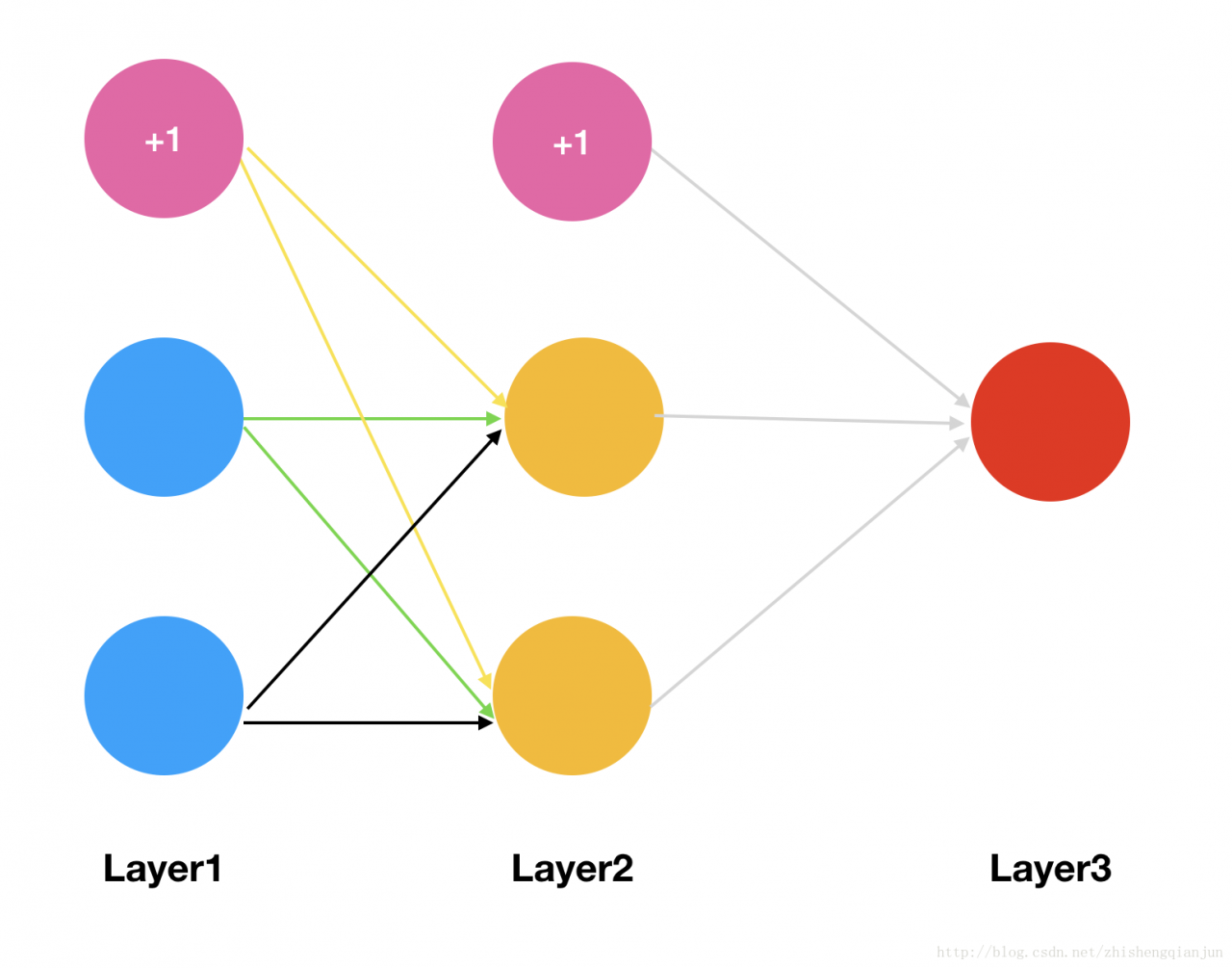
Then we will have two initial weight matrices:
θ1=[θ110θ120θ111θ121θ112θ122]θ2=[θ210θ211θ212]
We got the matrix above, and now we’re using
sigmoid
Function as the activation function to calculate the excitation of each layer of the network (assuming that we have only one sample, the input is
x1,x2,
The output is
y
);
The first level is input, and the incentive is the eigenvalue of the sample
a1=⎡⎣⎢⎢x0x1x2⎤⎦⎥⎥
x0
Is the bias term, which is 1
The second layer is the hidden layer. The excitation is obtained by multiplying the eigenvalue with the region, and then the sigmoid function is used to transform the region
a2
Before transformation
z2
:
z21z22z2a2a2=θ110∗x0+θ111∗x1+θ112∗x2=θ120∗x0+θ121∗x1+θ122∗x2=[z21z22]=sigmoid(z2)=⎡⎣⎢⎢⎢1a21a22⎤⎦⎥⎥⎥
In the above, we add a bias term at the end;
Next, the third layer is the output layer
z31z3a3a3=θ210∗a20+θ211∗a21+θ212∗a22=[z31]=sigmoid(z3)=[a31]
Because it is the output layer, there is no need to calculate further, so the bias term is not added;
The above calculation process, from input to output, is also called forward propagation.
Then, we write the formula of the loss function according to the loss function. Here, there is only one input and one output, so the loss function is relatively simple
Here, M = 1;
1
J(Θ)=−1m[y(i)klog((hΘ(x(i)))k)+(1−y(i)k)log(1−(hΘ(x(i)))k)]+λ2m∑l=1L−1∑i=1sl∑j=1sl+1(Θ(l)j,i)2=−1m[y∗log(a3)+(1−y)∗log(1−a3)]+λ2m∑l=1L−1∑i=1sl∑j=1sl+1(Θ(l)j,i)2
Note:
λ2m∑L−1l=1∑sli=1∑sl+1j=1(Θ(l)j,i)2
In fact, it is the sum of squares of all the weights. Generally, the one multiplied by the offset term will not be put in. This term is very simple. Ignore it for the time being, and do not write this term for the time being (this is regularization).
J(Θ)=−1m[y∗log(a3)+(1−y)∗log(1−a3)]
Then we get the above formula, and here we know if we want to ask for it
θ212
If we use the partial derivative of, we will find that this formula is actually a composite function,
y
It’s a constant. A3 is a constant
z3
Of
sigmoid
Function transformation, and
z3
then is
a2
Now that we have found where the weight is, we can start to find the partial derivative,
a3
finish writing sth.
s(z3)
Then, we get the following derivation:
∂J(Θ)∂θ212=−1m[y∗1s(z3)−(1−y)∗11−s(z3)]∗s(z3)∗(1−s(z3))∗a212=−1m[y∗(1−s(z3)−(1−y)∗s(z3)]∗a212=−1m[y−s(z3)]∗a212=1m[s(z3)−y]∗a212=1m[a3−y]∗a212
According to the above derivation, we can get the following formula:
1
∂J(Θ)∂θ210∂J(Θ)∂θ211=1m[a3−y]∗a210=1m[a3−y]∗a211
So, remember what I said earlier, we will seek the derivative from top to bottom and save the partial derivative of the current multiple subunits. According to the above formula, we know that the partial derivative of the second weight matrix can be obtained by
[a3−y]
It is obtained by multiplying the excitation of the previous layer of network and dividing it by the number of samples, so sometimes we call the difference as
δ3
Then, the partial derivatives of the second weight matrix are obtained by multiplying them in the form of matrix;
Now that we have obtained the partial derivatives of the second weight matrix, how can we find the partial derivatives of the first weight matrix?
For example, we’re going to
θ112
Partial derivation:
0
∂J(Θ)∂θ112=−1m[y∗1s(z3)−(1−y)∗11−s(z3)]∗s(z3)∗(1−s(z3))∗θ211∗s(z2)∗(1−s(z2))∗x2=−1m∗[a3−y]∗θ211∗s(z2)∗(1−s(z2))∗x2=−1m∗δ3∗θ211∗s(z2)∗(1−s(z2))∗x2
From the formula on the line, we can see that the derivative we saved can be directly multiplied. If there is a multi-layer network, in fact, the following process is the same as this one, so we get the formula:
if there is a multi-layer network, the following process is the same as this one
δ3δ2=a3−y=δ3∗(θ2)T∗s(z2)′
Because this network is three layers, so we can get all the partial derivatives. If it is multi-layer, the principle is the same. Multiply it continuously. Starting from the second formula, the following forms are the same.